III. The Forward Model

Previously, we assumed a Markovian forward model \[ \begin{align*} p_\theta(\mathbf{x}_{0:T}) & = p(\mathbf{x}_T)\prod_{t>0} p_\theta(\mathbf{x}_{t-1}|\mathbf{x}_t) \end{align*} \] In this section we'll place distributional assumptions on the above and derive a complete expression for the ELBO we'll optimize.

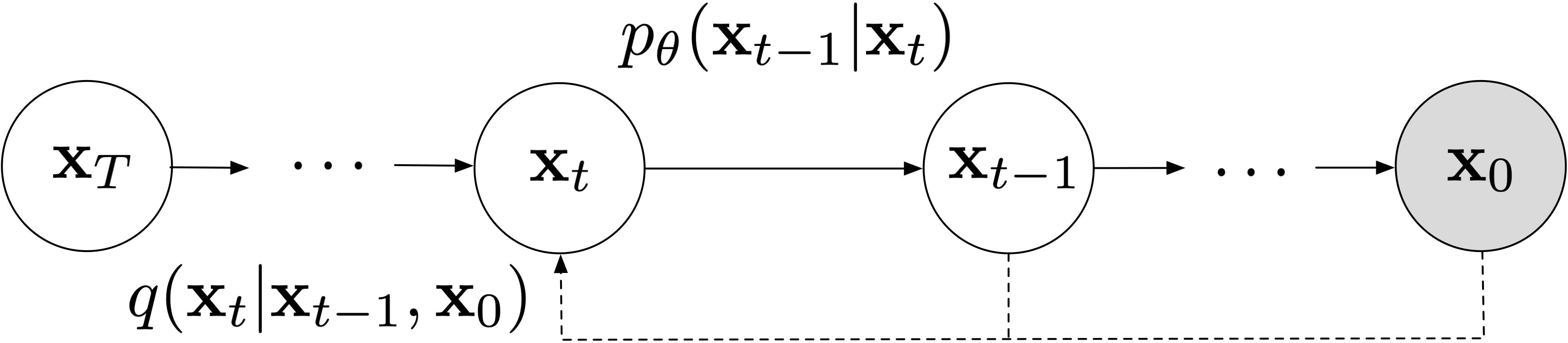
Define. For the forward model we'll use: \[ \begin{align*} p(\mathbf{x}_T) & = N(\mathbf{0},\mathbf{I})\\ p_\theta(\mathbf{x}_{t-1}|\mathbf{x}_t) & = q(\mathbf{x}_{t-1}|\mathbf{x}_t,f_\theta(\mathbf{x}_t)) \end{align*} \]

The prior here is chosen so that for any choice of \(\mathbf{x}_0\), we have \[ \begin{equation*} p(\mathbf{x}_T) \approx q(\mathbf{x}_T|\mathbf{x}_0) = N(\alpha_T\mathbf{x}_0,\sigma_T^2\mathbf{I}). \end{equation*} \] The approximation is reasonable because of our boundary assumption that \(\alpha_T\approx 0,\sigma_T \approx 1\).

Why is this desirable? Recall that one of the ELBO terms is to minimize \(D_\mathrm{KL}(\ q(\mathbf{x}_T|\mathbf{x}_0)\ \|\ p(\mathbf{x}_T)\ )\) which has no dependencies on learned parameters \(\theta\). By setting \(p(\mathbf{x}_T)\) in this way we're minimizing this term.

More importantly, let's move on to the Markov chain component. We're defining the forward model here as the backward model over \(\mathbf{x}_{t-1}\), given \(\mathbf{x}_t\) and a neural network's estimate of \(\mathbf{x}_0\) (where the network is given \(\mathbf{x}_t\) as input). For convenience, we repeat the definition of the true backward model, along with the expanded version of the forward model: \[ \begin{align*} q(\mathbf{x}_{t-1}|\mathbf{x}_t,\mathbf{x}_0) & = N\left(\alpha_{t-1}\mathbf{x}_0 + \sqrt{\sigma_{t-1}^2 - \gamma_t^2}\frac{\mathbf{x}_t-\alpha_t\mathbf{x}_0}{{\sigma_t}}, \gamma_t^2 \mathbf{I}\right)\\ p_\theta(\mathbf{x}_{t-1}|\mathbf{x}_t) & = N\left(\alpha_{t-1}f_\theta(\mathbf{x}_t) + \sqrt{\sigma_{t-1}^2 - \gamma_t^2}\frac{\mathbf{x}_t-\alpha_tf_\theta(\mathbf{x}_t)}{{\sigma_t}}, \gamma_t^2 \mathbf{I}\right) \end{align*} \] Remark. In principle we could have used any arbitrary distribution modeled via a neural network as the Markov chain in the forward model instead. For example, consider this strawman choice: \[ \begin{align*} p_\theta(\mathbf{x}_{t-1} | \mathbf{x}_t) = N(f_\theta(\mathbf{x}_t), \gamma_t^2\mathbf{I}). \end{align*} \]

We could in theory try to learn this model, but it would not leverage any of our prior knowledge about the assumed backward model. Instead, it's advantageous to constrain the neural network to only learning the component corresponding to \(\mathbf{x}_0\). (This was validated empirically in experiments by Ho et al. 2020.)

Remark. Notice the variance of the forward model is fixed to \(\gamma_t^2 \mathbf{I}\) and only the mean is learnable. There have been a few works that model the variance as learnable as well. We list a few below, though for simplicity we'll not explore them here.

Ho et al. (2020) tried allowing the variances \(\Sigma_\theta(\mathbf{x}_t,t)\) to be learned but found this led to worse reconstructions empirically.
Nichol and Dhariwal (2021) found that allowing it to be learned was necessary to achieve better log-likelihood estimates, but quality of reconstructions was not necessarily improved.

In the rest of this section we'll discuss possible choices for \(f_\theta(\mathbf{x}_t)\) i.e. the choice of parameterization.

\(\mathbf{x}_0\) Parameterization

Recall once again that the loss is defined, \[ \begin{align*} L_t(\mathbf{x}_0) & = \mathbb{E}_{\tilde{\mathbf{x}}_t\sim q(\mathbf{x}_t|\mathbf{x}_0)}\left[D_\mathrm{KL}(\ \underbrace{q(\mathbf{x}_{t-1}|\tilde{\mathbf{x}}_t, \mathbf{x}_0)}_{\text{groundtruth}}\ \|\ \underbrace{p_\theta(\mathbf{x}_{t-1}|\tilde{\mathbf{x}}_t)}_\text{prediction}\ )\right] \end{align*} \]

Next, recall that the KL divergence between \(q_1 = N(\boldsymbol\mu_1,\boldsymbol\Sigma_1)\) and \(q_2= N(\boldsymbol\mu_2,\boldsymbol\Sigma_2)\) in \(d\) dimensions has a closed form, \[ \begin{align*} D_\mathrm{KL}(\ q_1\ \|\ q_2\ ) &= \frac{1}{2}\left(\log \frac{|\boldsymbol\Sigma_2|}{|\boldsymbol\Sigma_1|} - d+\mathrm{tr}(\boldsymbol\Sigma^{-1}_2\boldsymbol\Sigma_1) + (\boldsymbol\mu_2-\boldsymbol\mu_1)^\top \boldsymbol\Sigma_2^{-1}(\boldsymbol\mu_2-\boldsymbol\mu_1)\right). \end{align*} \]

Because we fixed the variances of both \(p_\theta(\mathbf{x}_{t-1}|\mathbf{x}_t)\) and \(q(\mathbf{x}_{t-1}|\mathbf{x}_t,\mathbf{x}_0)\) (i.e. they're not learnable), all but the last term in the above expression are constant with respect to \(\theta\). Moreover, the fact that they're specifically fixed to \(\gamma_t^2 \mathbf{I}\) simplifies the math quite a bit. In the case where \(\boldsymbol\Sigma_1 = \boldsymbol\Sigma_2\), we have \[ \begin{align*} D_\mathrm{KL}(\ q_1\ \|\ q_2\ ) &= \frac{1}{2} (\boldsymbol\mu_2-\boldsymbol\mu_1)^\top \boldsymbol\Sigma_2^{-1}(\boldsymbol\mu_2-\boldsymbol\mu_1). \end{align*} \] Result. We can write the ELBO loss term as the following (note the \(\tilde{\mathbf{x}}_t\) terms cancel out on the third line below). \[ \begin{align*} L_t(\mathbf{x}_0) & = \mathbb{E}_{\tilde{\mathbf{x}}_t\sim q(\mathbf{x}_t|\mathbf{x}_0)}\left[D_\mathrm{KL}(\ \underbrace{q(\mathbf{x}_{t-1}|\tilde{\mathbf{x}}_t, \mathbf{x}_0)}_{\text{groundtruth}}\ \|\ \underbrace{p_\theta(\mathbf{x}_{t-1}|\tilde{\mathbf{x}}_t)}_\text{prediction}\ )\right]\\ & = \frac{1}{2\gamma_t^2}\mathbb{E}_{\tilde{\mathbf{x}}_t\sim q(\mathbf{x}_t|\mathbf{x}_0)}\left\| \alpha_{t-1}(\mathbf{x}_0 -f_\theta(\tilde{\mathbf{x}}_t)) + \frac{1}{\sigma_t}\sqrt{\sigma_{t-1}^2 - \gamma_t^2}(\tilde{\mathbf{x}}_t - \alpha_t\mathbf{x}_0 - \tilde{\mathbf{x}}_t + \alpha_t f_\theta(\tilde{\mathbf{x}}_t))\right\|^2\\ & = \frac{1}{2\gamma_t^2}\mathbb{E}_{\tilde{\mathbf{x}}_t\sim q(\mathbf{x}_t|\mathbf{x}_0)}\left\| \alpha_{t-1}(\mathbf{x}_0 -f_\theta(\tilde{\mathbf{x}}_t)) - \frac{\alpha_t}{\sigma_t}\sqrt{\sigma_{t-1}^2 - \gamma_t^2}(\mathbf{x}_0 - f_\theta(\tilde{\mathbf{x}}_t))\right\|^2\\ & = \frac{1}{2\gamma_t^2}\mathbb{E}_{\tilde{\mathbf{x}}_t\sim q(\mathbf{x}_t|\mathbf{x}_0)}\left\|\left(\alpha_{t-1}-\frac{\alpha_t}{\sigma_t}\sqrt{\sigma_{t-1}^2-\gamma_t^2}\right)(\mathbf{x}_0 - f_\theta(\tilde{\mathbf{x}}_t))\right\|^2\\ & = \underbrace{\frac{1}{2\gamma_t^2}\left(\alpha_{t-1}-\frac{\alpha_t}{\sigma_t}\sqrt{\sigma_{t-1}^2-\gamma_t^2}\right)^2}_{\omega_t}\mathbb{E}_{\tilde{\mathbf{x}}_t\sim q(\mathbf{x}_t|\mathbf{x}_0)}\left\|\underbrace{\mathbf{x}_0}_{\text{true denoised}} - \underbrace{f_\theta(\tilde{\mathbf{x}}_t)}_\text{predicted denoised}\right\|^2\\ & = \omega_t\mathbb{E}_{\tilde{\mathbf{x}}_t\sim q(\mathbf{x}_t|\mathbf{x}_0)}\left\|\mathbf{x}_0 - f_\theta(\tilde{\mathbf{x}}_t)\right\|^2 \end{align*} \]

For brevity (because we will re-use this equation later on), we hereon denote the weighting coefficient out front as \(\omega_t\), where \[ \begin{align*} \omega_t \triangleq \frac{1}{2\gamma_t^2}\left(\alpha_{t-1}-\frac{\alpha_t}{\sigma_t}\sqrt{\sigma_{t-1}^2-\gamma_t^2}\right)^2 \end{align*} \] In this setup we can interpret the neural network \(f_\theta(\tilde{\mathbf{x}}_t)\) as directly regressing the de-noised \(\mathbf{x}_0\).

\(\boldsymbol\epsilon\) Parameterization

Instead of predicting the true de-noised observation \(\mathbf{x}_0\), we can take advantage of how we're taking Monte Carlo samples and predict \(\boldsymbol\epsilon_t\), which is the noise that was added to \(\mathbf{x}_0\) to produce the sample \(\tilde{\mathbf{x}}_t\). Recall that we're drawing samples \[ \begin{align*} \tilde{\mathbf{x}}_t & = \alpha_t\mathbf{x}_0 + \sigma_t\boldsymbol\epsilon_t, & \boldsymbol\epsilon_t &\sim N(\mathbf{0}, \mathbf{I}). \end{align*} \] which means that we can equivalently write \[ \begin{align*} \mathbf{x}_0 & = \frac{1}{\alpha_t}(\tilde{\mathbf{x}}_t - \sigma_t\boldsymbol\epsilon_t), & \boldsymbol\epsilon_t &\sim N(\mathbf{0}, \mathbf{I}). \end{align*} \]

Here we'll define the neural network prediction of \(\mathbf{x}_0\) in a very specific way, \[ \begin{align*} f_\theta(\tilde{\mathbf{x}}_t) & = \frac{1}{\alpha_t}(\tilde{\mathbf{x}}_t - \sigma_tg_\theta(\tilde{\mathbf{x}}_t)) \approx \boldsymbol\epsilon_t \end{align*} \]

where the neural network parameters all lie in \(g_\theta(\tilde{\mathbf{x}}_t)\) which approximates the noise \(\boldsymbol\epsilon_t\).

Result. Here the ELBO loss term is (note the \(\tilde{\mathbf{x}}_t\) terms cancel out on the third line below) \[ \begin{align*} L_t(\mathbf{x}_0) & = \omega_t\mathbb{E}_{\tilde{\mathbf{x}}_t\sim q(\mathbf{x}_t|\mathbf{x}_0)}\left\|\underbrace{\mathbf{x}_0}_{\text{true denoised}} - \underbrace{f_\theta(\tilde{\mathbf{x}}_t)}_\text{predicted denoised}\right\|^2\\ & = \omega_t\mathbb{E}_{\tilde{\mathbf{x}}_t\sim q(\mathbf{x}_t|\mathbf{x}_0)}\left\|\frac{1}{\alpha_t}(\tilde{\mathbf{x}}_t - \sigma_t \boldsymbol\epsilon_t) - \frac{1}{\alpha_t}(\tilde{\mathbf{x}}_t - \sigma_tg_\theta(\tilde{\mathbf{x}}_t))\right\|^2\\ & = \omega_t\mathbb{E}_{\tilde{\mathbf{x}}_t\sim q(\mathbf{x}_t|\mathbf{x}_0)}\left\|\frac{\sigma_t}{\alpha_t}(\boldsymbol\epsilon_t-g_\theta(\tilde{\mathbf{x}}_t ))\right\|^2\\ & = \omega_t\frac{\sigma_t^2}{\alpha_t^2}\mathbb{E}_{\tilde{\mathbf{x}}_t\sim q(\mathbf{x}_t|\mathbf{x}_0)}\left\|\underbrace{\boldsymbol\epsilon_t}_\text{true noise}-\underbrace{g_\theta(\tilde{\mathbf{x}}_t )}_\text{predicted noise}\right\|^2\\ \end{align*} \] Result. The \(\boldsymbol\epsilon\) parameterization has a convenient interpretation as regressing a scaled version of score of the distribution \(q(\mathbf{x}_t|\mathbf{x}_0)\). From the definition of Gaussian log-likelihood it follows that \[ \begin{align*} \nabla_{\mathbf{x}_t}\log q(\mathbf{x}_t|\mathbf{x}_0) & = -\nabla_{\mathbf{x}_t}\left(\frac{\|\mathbf{x}_t-\alpha_t\mathbf{x}_0\|^2}{2\sigma_t^2} +(\dots)\right)= \frac{-1}{\sigma_t^2}\left(\mathbf{x}_t-\alpha_t\mathbf{x}_0\right) \end{align*} \] which means we can write \[ \begin{align*} \boldsymbol\epsilon_t & = \frac{-1}{\sigma_t}(\mathbf{x}_t-\alpha_t\mathbf{x}_0) = -\sigma_t\nabla_{\mathbf{x}_t}\log q(\mathbf{x}_t|\mathbf{x}_0). \end{align*} \] This draws a connection to the score matching objective (Song and Ermon 2019).

\(\mathbf{v}\) Parameterization

In a subsequent section when discussing the noise schedule we'll define the velocity interpretation and parameterization. Read that section first and then return here. But suffice it to say here the neural network will be predicting \(\mathbf{v}_t\), the velocity at timestep \(t\).

Recall that the velocity is defined \[ \begin{align*} \mathbf{v}_t & = \alpha_t\boldsymbol\epsilon_t-\sigma_t\mathbf{x}_0, & \boldsymbol\epsilon_t &\sim N(\mathbf{0}, \mathbf{I}) \end{align*} \] and that we can equivalently write \[ \begin{align*} \mathbf{x}_0 & = \alpha_t\tilde{\mathbf{x}}_t-\sigma_t\mathbf{v}_t. \end{align*} \] Here we'll define the neural network prediction of \(\mathbf{x}_0\) as \[ \begin{align*} f_\theta(\tilde{\mathbf{x}}_t) & = \alpha_t\tilde{\mathbf{x}}_t-\sigma_t h_\theta(\tilde{\mathbf{x}}_t), \end{align*} \] where the neural network is now \(h_\theta(\tilde{\mathbf{x}}_t)\) which approximates the velocity \(\mathbf{v}_t\).

Result. Here the ELBO loss term is (note \(\tilde{\mathbf{x}}_t\) terms cancel out on the third line below) \[ \begin{align*} L_t(\mathbf{x}_0) & = \omega_t\mathbb{E}_{\tilde{\mathbf{x}}_t\sim q(\mathbf{x}_t|\mathbf{x}_0)}\left\|\underbrace{\mathbf{x}_0}_{\text{true denoised}} - \underbrace{f_\theta(\tilde{\mathbf{x}}_t)}_\text{predicted denoised}\right\|^2\\ & = \omega_t\mathbb{E}_{\tilde{\mathbf{x}}_t\sim q(\mathbf{x}_t|\mathbf{x}_0)}\left\| \alpha_t\tilde{\mathbf{x}}_t -\sigma_t\mathbf{v}_t - \alpha_t\tilde{\mathbf{x}}_t + \sigma_t\mathbf{v}_t\right\|^2\\ & = \omega_t\sigma_t^2\mathbb{E}_{\tilde{\mathbf{x}}_t\sim q(\mathbf{x}_t|\mathbf{x}_0)}\left\|\underbrace{\mathbf{v}_t}_{\text{true velocity}} -\underbrace{h_\theta(\tilde{\mathbf{x}}_t)}_{\text{predicted velocity}}\right\|^2 \end{align*} \]

Deriving predicted \(\mathbf{x}_0,\boldsymbol\epsilon,\mathbf{v}\) from each other

It's important to note that no matter which of the three parameterizations above we choose for the neural network, one prediction from the network implies the entire set of values for \(\mathbf{x}_0,\boldsymbol\epsilon,\mathbf{v}\). In other words, these values can all be derived from each other.

For example, suppose we choose the \(\mathbf{x}_0\) parameterization. Our neural network is \(f_\theta(\tilde{\mathbf{x}}_t)\). Then \[ \begin{align*} \hat{\mathbf{x}}_0(\mathbf{x_t}) & = f_\theta(\tilde{\mathbf{x}}_t) & \hat{\boldsymbol\epsilon}_t(\mathbf{x}_t)& = \frac{1}{\sigma_t}(\tilde{\mathbf{x}}_t - \alpha_tf_\theta(\tilde{\mathbf{x}}_t))&\hat{\mathbf{v}}_t(\tilde{\mathbf{x}}_t) & = \frac{1}{\sigma_t}(\alpha_t\tilde{\mathbf{x}}_t-f_\theta(\tilde{\mathbf{x}}_t)). \end{align*} \] Likewise, suppose we choose the \(\boldsymbol\epsilon\) parameterization. Our neural network is \(g_\theta(\tilde{\mathbf{x}}_t)\). Then \[ \begin{align*} \hat{\mathbf{x}}_0(\mathbf{x_t}) & = \frac{1}{\alpha_t}(\tilde{\mathbf{x}}_t - \sigma_t g_\theta(\tilde{\mathbf{x}}_t)) & \hat{\boldsymbol\epsilon}_t(\mathbf{x}_t)& = g_\theta(\tilde{\mathbf{x}}_t)&\hat{\mathbf{v}}_t(\tilde{\mathbf{x}}_t) & = \frac{1}{\alpha_t}(g_\theta(\tilde{\mathbf{x}}_t)-\sigma_t\tilde{\mathbf{x}}_t). \end{align*} \] Henceforth, we'll use notation \[ \begin{align*} \hat{\mathbf{x}}_0(\mathbf{x_t}) && \hat{\boldsymbol\epsilon}_t(\mathbf{x}_t)&&\hat{\mathbf{v}}_t(\mathbf{x}_t) \end{align*} \] to denote the predictions for these quantities irrespective of our choice of neural network parameterization. (It's implied that these have parameters \(\theta\), even though it's not explicit in the notation.)

Simple Losses

In practice, for each of the parameterizations it is common to completely ignore the corresponding weighting coefficient on the ELBO and use one these simple losses \(L_t'(\mathbf{x}_0)\) instead. \[ \begin{align*} (\mathbf{x}_0\text{ parameterization})\quad& L'_t(\mathbf{x}_0) = \mathbb{E}_{\tilde{\mathbf{x}}_t\sim q(\mathbf{x}_t|\mathbf{x}_0)}\left\|\mathbf{x}_0 - f_\theta(\tilde{\mathbf{x}}_t)\right\|^2\\ (\boldsymbol\epsilon \text{ parameterization})\quad & L'_t(\mathbf{x}_0) = \mathbb{E}_{\tilde{\mathbf{x}}_t\sim q(\mathbf{x}_t|\mathbf{x}_0)}\left\|\boldsymbol\epsilon - g_\theta(\tilde{\mathbf{x}}_t)\right\|^2\\ (\mathbf{v} \text{ parameterization})\quad & L'_t(\mathbf{x}_0) = \mathbb{E}_{\tilde{\mathbf{x}}_t\sim q(\mathbf{x}_t|\mathbf{x}_0)}\left\|\mathbf{v} - h_\theta(\tilde{\mathbf{x}}_t)\right\|^2\\ \end{align*} \] Remark. Using a simple loss implies that the choice of \(\gamma_t\) actually doesn't matter in the training procedure at all. This is because the only impact it has is on the coefficient \(\omega_t\) which is ignored in the smple loss.

Remark. Even though all the derivations for the ELBO \(L_t(\mathbf{x}_0)\) in the previous section are equivalent to each other (regardless of which parameterization is used), each parameterization leads to a different simple loss.

Why choose one of these losses? Empirically, in the case of \(\boldsymbol\epsilon\)-prediction at least, Ho et al. 2020 found the simple loss to perform better than the actual ELBO \(L_t(\mathbf{x}_0)\).

Result. Using a simple loss is equivalent to applying a weight to each term in the ELBO, where the weight is the reciprocal of the actual coefficient out front in the ELBO. We can summarize with the following table.

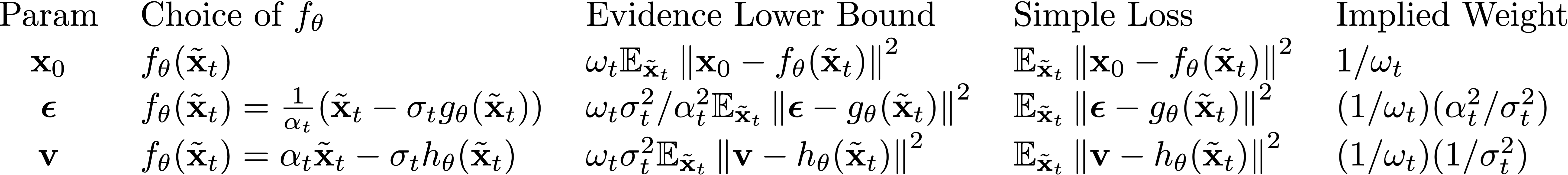
For example, two of the most common parameterizations used today are the \(\boldsymbol\epsilon\) parameterization and the \(\mathbf{x}_0\) parameterization with their corresponding simple losses. From the table above, it is easy to see that use of one is equivalent to use of the other but applying an implied weighting factor of \(\alpha_t^2/\sigma_t^2\) (i.e. the SNR). (Equivalence here is from a loss perspective, of course from a neural network learning perspective there are differences as well. One choice of parameterization may be easier for a network to learn than another).

Remark. Why is it theoretically justified to optimize these simple losses instead of the actual ELBO? Song et al. (2021) argued with the following. Suppose the parameters for \(f_\theta(\tilde{\mathbf{x}}_t)\) are not shared across \(t\). Then optimizing a simple loss \(L'_t(\mathbf{x}_0)\) will lead to the same solution as optimizing the actual ELBO \(L_t(\mathbf{x}_0)\), because optimizing each term independently is the same as optimizing the weighted sum. So if our model is sufficiently powerful, in theory ignoring these weighting factors is roughly okay.

Pseudocode. We can update our pseudocode accordingly, where below we assume use of the simple loss.

def compute_L_t(x_0):
    t = sample_t(lower=1, upper=T)
    eps = randn_like(x_0)
    monte_carlo_x_t = alpha_t * x_0 + sigma_t * eps
    target = (x_0) OR (eps) OR (sigma_t * eps - alpha_t * x_0)  # this line changed
    pred = neural_network(monte_carlo_x_t, t)  # this line changed
    loss = (target - pred) ** 2
    return loss