IX. Karras Parameterization
One of the most impactful papers on diffusion models is Karras et al. 2022, "Elucidating the Design Space of Diffusion-Based Generative Models". Building on top of the SDE framework for diffusion models, the authors identified a design space consisting of:
- The network parameterization.
- The loss weighting.
- The training-time distribution over \(\sigma\) to draw noisy samples.
- The inference-time discretization over \(\sigma\) to take solver steps over.
- The choice of ODE integration space.
- The choice of ODE solver.
On this page we'll explore the first four of the above contributions. We'll leave the last two to the subsequent page on advanced solvers.
Throughout this section we'll adopt the generic notation of a Variance-Exploding SDE. We note that, as previously shown, diffusion models are a special case of such SDEs. But on this page focusing on the general case will simplify the notation.
Specifically, we model the marginal distribution as \[ \begin{align*} \mathbf{x}_t \sim p_t(\mathbf{x}_t| \mathbf{x}_0) = \mathbf{x}_0 + \sigma_t\boldsymbol\epsilon_t,\quad\quad\boldsymbol\epsilon_t \sim N(\mathbf{0}, \mathbf{I}). \end{align*} \]
Recall (from the discrete score matching section) that the corresponding score is \[ \begin{align*} \underbrace{\nabla_{\mathbf{x}_t} p_t(\mathbf{x}_t|\mathbf{x}_0)}_{\approx\ s_\theta(\mathbf{x}_t)} & = \frac{-1}{\sigma_t^2}(\mathbf{x}_t - \mathbf{x}_0) = \frac{-1}{\sigma_t} \underbrace{\boldsymbol\epsilon_t}_{\approx\ \hat{\boldsymbol\epsilon}(\mathbf{x}_t)}. \end{align*} \] In terms of notation, we'll approximate the score with \(s_\theta(\mathbf{x})\) and the noise with \(\hat{\boldsymbol\epsilon}_\theta(\mathbf{x})\), noting that both are valid modeling choices for the neural network.
Moreover, we'll assume throughout that \(\text{Var}[\mathbf{x}_0] = \sigma_\text{data}^2\).
Training and Inference Noise Distributions
In continous time, we no longer sample from a discrete set of \(\sigma_t\). Instead, at training time we sample from a continuous distribution over \(\sigma \in [\sigma_\text{min}, \sigma_\text{max}]\). Meanwhile at inference time we choose a discrete set of \(\sigma\) to take steps in. There are several possible choices for how to do so.
Throughout this section we'll express distributions over \(\log\sigma\) as in the figure below.

Cosine (Hyperbolic Secant) Schedule.
We first draw an analogy to the cosine schedule with which we're familiar. We'll handle the general case where we shift the log-SNR by \(+2\log \kappa\). Recall that in this setup we can express (assuming \(\sigma_\text{data}=1\)) \[ \begin{align*} \mathrm{SNR}_t^{-\frac{1}{2}} & = \sigma_t = \frac{1}{\kappa}\frac{\sin\theta_t}{\cos\theta_t} = \frac{\tan \theta_t}{\kappa}. \end{align*} \] The cosine schedule is linearly spaced in \(\theta_t \in [0, \frac{\pi}{2}]\). Because it's linearly spaced, we can interpret it as an inverse CDF, i.e. \(\sigma_t\) as the transformation of a uniform random variable in \(\theta_t\).
Therefore, we can express the inverse CDF over \(\log\sigma\) as \[ \begin{align*} F^{-1}(p) & = \log \tan\left(\frac{\pi}{2}p\right)-\log\kappa,\quad\quad p\in[0,1]. \end{align*} \] This is equivalent to the inverse CDF of a Hyperbolic Secant distribution scaled by \(\frac{\pi}{2}\) and subsequently shifted by \(-\log \kappa\). \[ \begin{align*} \log\sigma & \sim \frac{\pi}{2}\text{HypSecant}() - \log\kappa\\ \frac{2}{\pi}\left(\log \sigma + \log \kappa\right)& \sim \text{HypSecant}() \end{align*} \]
Recall that a Hyperbolic Secant distribution has PDF \(f(x) =\frac{1}{2}\mathrm{sech}\left(\frac{\pi}{2}x\right)\). Using the change of variables formula, we can conclude that the PDF over \(\log\sigma\) is \[ \begin{align*} f(\log\sigma) & = \frac{1}{\pi}\mathrm{sech}\left(\log\sigma+\log\kappa\right). \end{align*} \] We can repeat this exercise in \(\sigma\) space as well, and we find that (Johnson et al. 1994) [Footnote 1] \[ \begin{align*} \sigma & \sim \text{HalfCauchy}(1/\kappa). \end{align*} \] Note that the Hyperbolic Secant distribution has heavier tails than the Normal distribution.
Normal Schedule.
The Normal schedule is a very simple schedule proposed by Karras et al. 2022. Empirically this was found by the authors to be the most competitive training schedule for images.
It's defined with the hyper-parameters specified below, \[ \begin{align*} \log \sigma_t &\sim N(\mu,\gamma)& \mu & = -1.2&\gamma&=1.2. \end{align*} \] The PDF is the familiar Gaussian PDF, \[ \begin{align*} f(\log\sigma) & = \frac{1}{\sqrt{2\pi\gamma^2}}e^{-\frac{(\log\sigma - \mu)}{2\gamma^2}}. \end{align*} \] Exponential Schedule.
The Exponential Schedule is the inference-time schedule proposed by Karras et al. 2022. Empirically the authors found it to be the most competitive inference schedule for images.
It's not actually a distribution used for sampling, but a distribution we use at inference time by evaluating at equal quantiles of the inverse CDF. For example, for 10 inference steps we would evaluate at the 100th, 90th, 80th, ... 20th, 10th percentiles.
The inverse CDF over \(\sigma\) is parameterized by a constant \(\rho \triangleq 7\) and a maximum \(\sigma_\text{max}\). To make this more familiar, we can convert it to an inverse CDF over \(-\log\sigma\) as below [Footnote 2]. \[ \begin{align*} F^{-1}(p) & = (p\ \sigma_\text{max}^{1/\rho})^\rho & \text{for } & \sigma\\ F^{-1}(p) & = -\rho\log(1-p) - \log\sigma_\text{max} & \text{for } & -\log\sigma \end{align*} \] This is equivalent to the inverse CDF for a shifted exponential distribution with rate \(1/\rho\). Specifically, we can write the associated PDF over \(\log \sigma\) as \[ \begin{align*} -(\log\sigma - \log\sigma_\text{max}) & \sim \mathrm{Exp}(1/\rho)\\ f(\log \sigma) & = \frac{1}{\rho} e^{\frac{1}{\rho}(\log\sigma - \log \sigma_\text{max})}. \end{align*} \]
This PDF can be made further precise by accounting for \(\sigma_\text{min}\) [Footnote 3].
Choice of Network Parameterization
Previously we've discussed three possible choices: \(\mathbf{x}_0\), \(\mathbf{v}\), and \(\boldsymbol\epsilon\) prediction. These can all be instantiated as specific cases of the following parameterization.
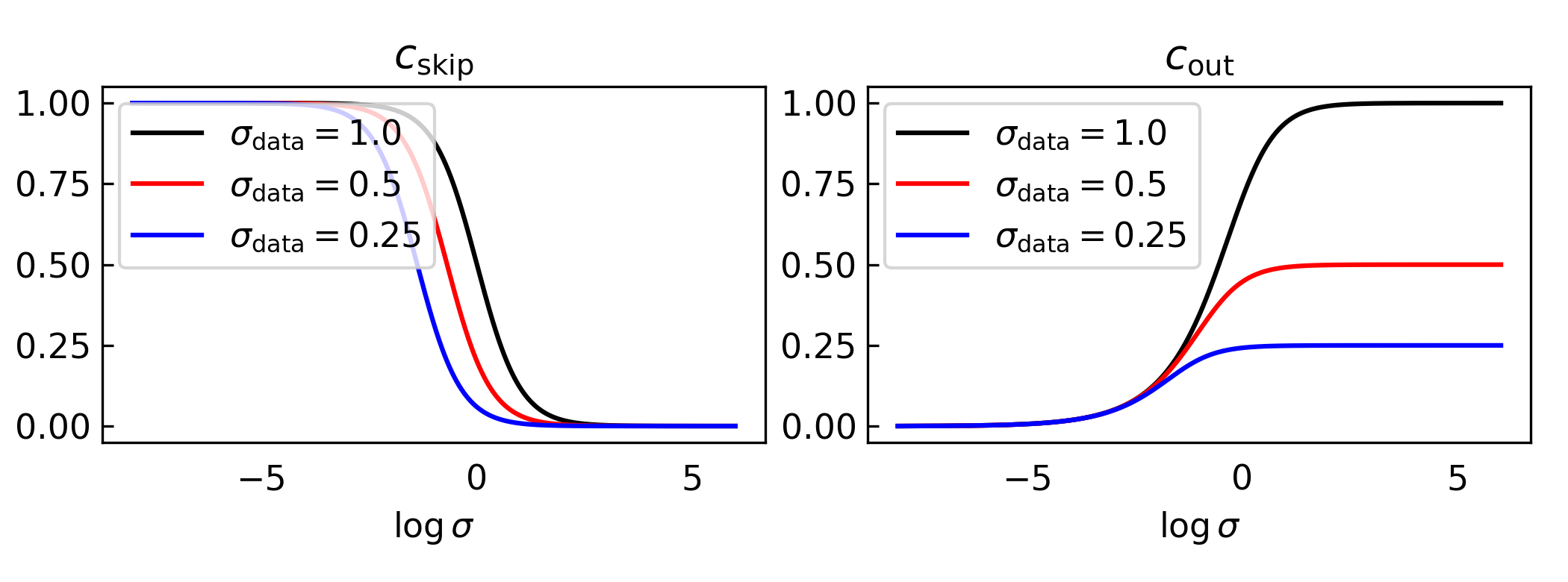
Define. The Karras network parameterization tries to predict denoised observations \(\mathbf{x}_0\) using \[ \begin{align*} \hat{\mathbf{x}}_0(\mathbf{x},\sigma;\theta) & = c_\text{skip}\mathbf{x}+c_\text{out}f_\theta(c_\text{in}\mathbf{x},\sigma) \end{align*} \] where \(c_\text{skip}, c_\text{out}, c_\text{in}\) are scalars that depend on \(\sigma\) and \(f_\theta\) is the neural network.
Remark. Setting \((c_\text{skip} = 0,c_\text{out}=1)\) recovers \(\mathbf{x}_0\) prediction. Setting \((c_\text{skip}=1, c_\text{out}=-\sigma\)) recovers \(\boldsymbol\epsilon\) prediction.
Result. With the Karras network parameterization, the score-matching loss function (with loss weights \(w_\sigma\) we'll soon discuss) simplifies to \[ \begin{align*} J(\theta) = w_\sigma\|\mathbf{x}_0-\hat{\mathbf{x}}_0(\mathbf{x},\sigma;\theta)\|^2 & = w_\sigma c_\text{out}^2\left\|\underbrace{f_\theta(c_\text{in}\mathbf{x},c_\text{noise}\sigma_t)}_\text{network output} - \underbrace{\frac{1}{c_\text{out}}\left(c_\text{skip} \sigma \boldsymbol\epsilon + (1-c_\text{skip})\mathbf{x}_0\right)}_\text{network target}\right\|^2 \end{align*} \] Proof. This follows from a bit of algebra, and plugging in the fact that \(\mathbf{x} = \mathbf{x}_0 + \sigma\boldsymbol\epsilon\). It's extremely uninteresting to write out fully.
Setup. We now walk through how to set the constants in the parameterization.
- Require the network input to have unit variance. \[ \begin{align*} \text{Var}[c_\text{in}\mathbf{x}] & = c_\text{in}^2\left(\sigma_\text{data}^2+ \sigma^2\right) = 1\\ c_\text{in} & = \frac{1}{\sqrt{\sigma_\text{data}^2+\sigma^2}} \end{align*} \]
- Require the network target to have unit variance. \[ \begin{align*} \text{Var}\left[\frac{1}{c_\text{out}}\left(c_\text{skip} \sigma \boldsymbol\epsilon + (1-c_\text{skip})\mathbf{x}_0\right)\right] &= \frac{1}{c_\text{out}^2}\left(c_\text{skip}^2\sigma^2 + (1-c_\text{skip})^2\sigma_\text{data}^2\right) = 1\\ c_\text{out}^2 & = \left(c_\text{skip}^2\sigma^2 + (1-c_\text{skip}^2)\sigma_\text{data}^2\right) \end{align*} \]
- Pick \(c_\text{skip}\) to minimize \(c_\text{out}\). This is a univariate convex optimization problem. \[ \begin{align*} \frac{d}{d c_\text{skip}} c_\text{out}^2 & = 2c_\text{skip}\sigma^2 -2(1-c_\text{skip}^2)\sigma_\text{data}^2 = 0\\ c_\text{skip} & = \frac{\sigma_\text{data}^2}{\sigma^2 + \sigma_\text{data}^2} \implies c_\text{out} = \frac{\sigma\ \sigma_\text{data}}{\sqrt{\sigma^2+\sigma_\text{data}^2}} \end{align*} \]
Remark. Setting \(\sigma_\text{data}=1\) with the above choices for \(c_\text{skip}, c_\text{out}\) recovers \(\mathbf{v}\) parameterization.
Below we plot what these choices look like for different levels of \(\sigma_\text{data}\).
Choice of Loss Weighting
We've already seen that the loss function in this setup is \[ \begin{align*} J(\theta) & = w_\sigma\|\mathbf{x}_0-\hat{\mathbf{x}}_0(\mathbf{x},\sigma;\theta)\|^2\\ & = w_\sigma c_\text{out}^2\left\|\underbrace{f_\theta(c_\text{in}\mathbf{x},c_\text{noise}\sigma_t)}_\text{network output} - \underbrace{\frac{1}{c_\text{out}}\left(c_\text{skip} \sigma \boldsymbol\epsilon + (1-c_\text{skip})\mathbf{x}_0\right)}_\text{network target}\right\|^2 \end{align*} \]
where we know both network output and target have constant variance over \(\sigma\).
Remark. We can connect to a few different losses we've seen before \[ \begin{align*} w_\sigma & = 1 & &&& \mathbf{x}_0 \text{ prediction simple loss}\\ w_\sigma & = \sigma_\text{data}^2/\sigma^2 & &&& \boldsymbol\epsilon \text{ prediction simple loss}\\ w_\sigma & = \text{min}(\sigma_\text{data}^2/\sigma^2, 5) &&&& \text{Min-SNR weighting} \end{align*} \] Define. The Karras choice of weighting picks \(w_\sigma\) so that the effective network weight \(w_\sigma c_\text{out}^2\) is uniform. \[ \begin{align*} w_\sigma c_\text{out}^2 & = 1\\ w_\sigma & = \frac{\sigma^2 + \sigma_\text{data}^2}{(\sigma\ \sigma_\text{data})^2} \end{align*} \] Remark. Observe that when \(\sigma_\text{data}=1\), this is equivalent to \(\mathbf{v}\) prediction simple loss.
[Footnote 1] Recall that if \(X\sim \text{Cauchy}(0, \gamma)\) then \(|X|\sim\text{HalfCauchy}(\gamma)\).
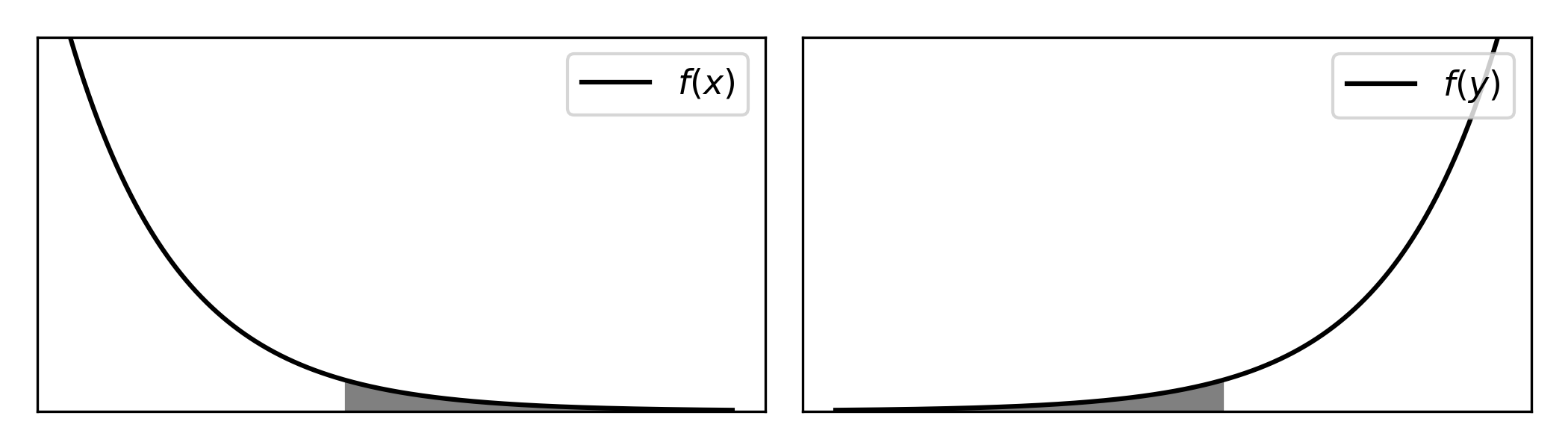
[Footnote 2] This relies on the following. Suppose random variables \(X \sim F(x)\) and \(Y=-X\), then we have \[ \begin{align*} \underbrace{F(y)}_{\text{over }Y} & = 1 - \underbrace{F(-y)}_{\text{over }X} & \quad\quad\underbrace{F^{-1}(p)}_{\text{over } Y} &= -\underbrace{F^{-1}(1-p)}_{\text{over }X} \end{align*} \] For intuition, see the figure below and imagine the mapping from \(p\in[0,1]\) to samples.
[Footnote 3] For the other distributions above we ignored the truncation of the left-side tail by \(\sigma_\text{min}\). However, for the Exponential schedule this tail is actually significant and we need to rescale by the partition constant induced by the tail. To do so, we can write \[ \begin{align*} f(\log\sigma) & = \frac{1}{Z\rho }e^{\frac{1}{\rho}(\log \sigma - \log\sigma_\text{max})}\\ Z & = 1 - e^{-\rho(\sigma_\text{max}- \sigma_\text{min})}. \end{align*} \]