V. The Noise Schedule

Choice of noise schedule \(\{\boldsymbol\alpha, \boldsymbol\sigma\}\) has a significant impact on the quality of a learned model and is often the single most important hyper-parameter to tune. Recall the assumptions we made.

Variance Preserving: \(\alpha_t^2 + \sigma_t^2 = 1\).
Monotonic: \(\alpha_t > \alpha_{t+1}\) and consequently \(\sigma_t < \sigma_{t=1}\).
Boundary Conditions: \(\alpha_0 = 1,\sigma_0=0,\alpha_T\approx 0,\sigma_T\approx 1\).

It's easy to see there are actually only \(T-1\) degrees of freedom in the noise schedule. In particular there's some redundancy because \(\alpha_t\) and \(\sigma_t\) can always be derived from one another. (We keep both symbols around to help simplify notation).

Even though the noise schedule isn't directly used to weight the loss (due to our use of simple losses), it does affect the Monte Carlo samples \(\tilde{\mathbf{x}}_t\sim q(\mathbf{x}_t|\mathbf{x}_0)\) in the optimization process.

Commonly Used Options

For sake of concreteness and to give a bit of intuition, we'll introduce a few options.

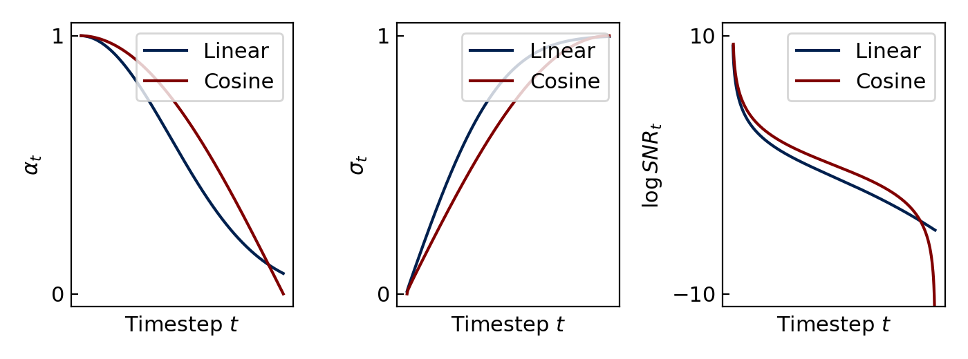
Cosine schedule (Nichol and Dhariwal 2021). [Footnote 1] \[ \begin{align*} \alpha_t &= \cos\left(\frac{\pi t}{2T}\right)&\sigma_t & = \sin\left(\frac{\pi t}{2T}\right) \end{align*} \] This is the most commonly used schedule in the literature.
Linear schedule (Ho et al. 2020). \[ \begin{align*} \beta_s &= \frac{s}{T}(0.02-0.0001)+0.0001&\alpha_t &= \sqrt{\prod_{s=1}^t(1-\beta_s)} & \sigma_t = 1-\alpha_t \end{align*} \] This schedule is no longer commonly used, and is included mostly for historical purposes.

Angular Interpretation

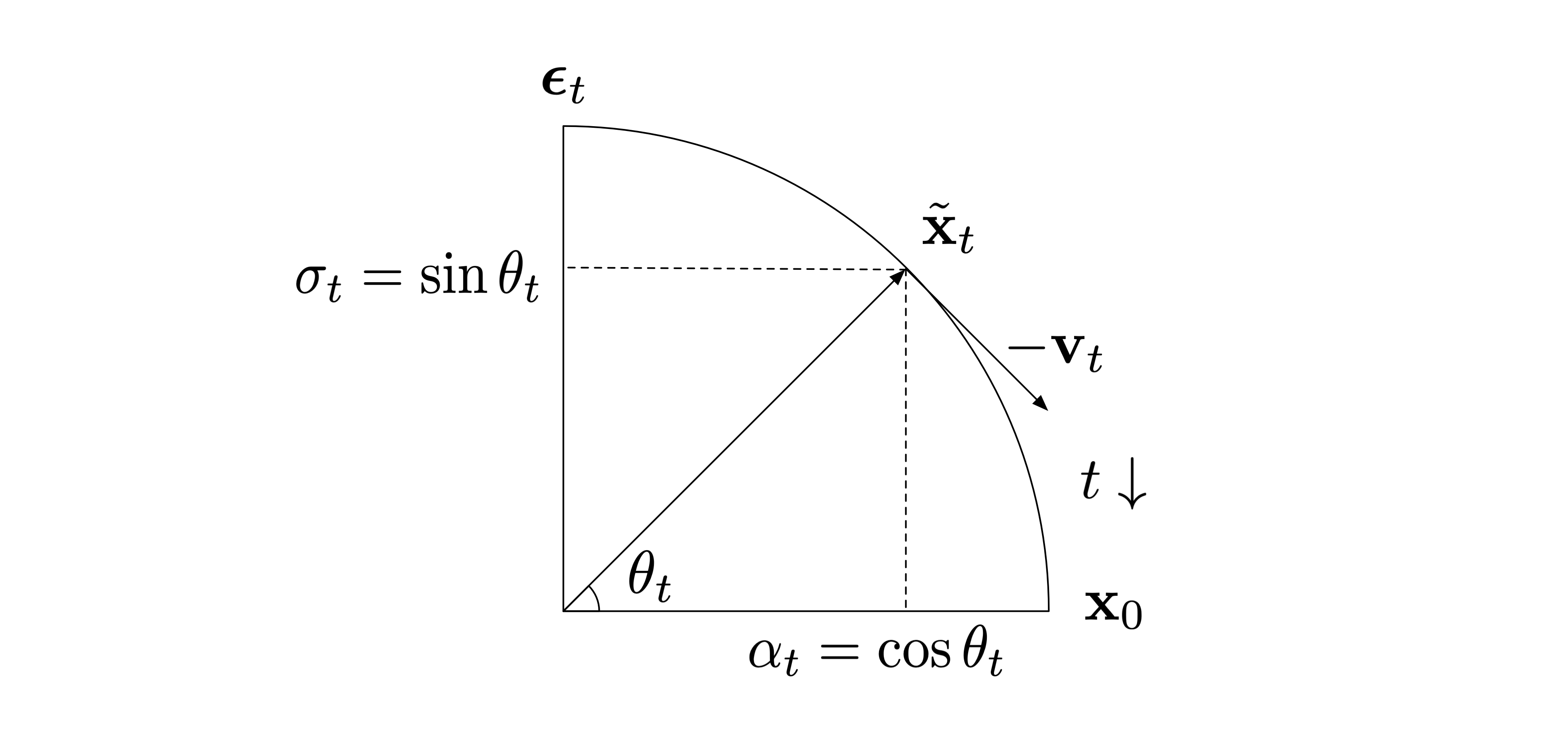
With the variance preserving assumption, we can interpret the noise schedule as the specification for a series of increasing angles \(\theta_t\) in the first quadrant (Salimans and Ho 2022), where \[ \begin{align*} \theta_t = \tan^{-1}(\sigma_t/\alpha_t)\quad\quad \alpha_t = \cos\theta_t \quad\quad \sigma_t = \sin \theta_t. \end{align*} \]

For example, with a cosine schedule we have \(\theta_t = \frac{\pi t}{2T}\) which linearly discretizes the first quadrant from 0 to \(\pi/2\).

The figure below exhibits this angular interpretation, noting that \(\tilde{\mathbf{x}}_t\) is a convex combination of \(\mathbf{x}_0\) and \(\boldsymbol\epsilon_t\) that interpolates between the two depending on \(t\) (and the corresponding angle \(\theta_t\)).

Velocity Parameterization

Define. The velocity is the derivative of \(\tilde{\mathbf{x}}_t\) with respect to \(\theta\), \[ \begin{align*} \mathbf{v}_t & = \frac{d}{d\theta}\tilde{\mathbf{x}}_t = \frac{d}{d\theta}(\alpha_t \mathbf{x}_0 + \sigma_t \boldsymbol\epsilon_t)\\ & = \frac{d}{d\theta}((\cos\theta)\mathbf{x}_0 +(\sin\theta)\boldsymbol\epsilon_t)\\ & = (\cos\theta) \boldsymbol\epsilon_t - (\sin\theta)\mathbf{x}_0\\ & = \alpha_t \boldsymbol\epsilon_t - \sigma_t\mathbf{x}_0 \end{align*} \]

Remark. Visually, the velocity is depicted as the tangent to the arc swept out by \(\tilde{\mathbf{x}}_t\) in the previous figure. Notice that in the \(\{\mathbf{x}_0,\boldsymbol\epsilon_t\}\) basis, the length of both \(\mathbf{v}_t\) and \(\tilde{\mathbf{x}}_t\) are 1.

Result. There are a couple helpful identities we can derive from this definition of velocity, to express \(\mathbf{x}_0\) and \(\boldsymbol\epsilon_t\) in terms of \(\tilde{\mathbf{x}}_t\) and \(\mathbf{v}_t\). \[ \begin{align*} \mathbf{x}_0 & = \alpha_t\tilde{\mathbf{x}}_t - \sigma_t\mathbf{v}_t\\ \boldsymbol\epsilon_t & = \sigma_t\tilde{\mathbf{x}}_t + \alpha_t\mathbf{v}_t \end{align*} \] Proof. Starting from the key result, we can write the following. \[ \begin{align*} \tilde{\mathbf{x}}_t & = \alpha_t \mathbf{x}_0 + \sigma_t\boldsymbol\epsilon_t\\ \tilde{\mathbf{x}}_t& = \alpha_t\mathbf{x}_0 + \frac{\sigma_t}{\alpha_t}\left(\mathbf{v}_t + \sigma_t\mathbf{x}_0)\right) \tag{from the definition above}\\ & = \left(\alpha_t + \frac{\sigma_t^2}{\alpha_t}\right)\mathbf{x}_0 +\frac{\sigma_t}{\alpha_t}\mathbf{v}_t \tag{re-arrange}\\ \alpha_t\tilde{\mathbf{x}}_t & = \mathbf{x}_0 + \sigma_t\mathbf{v}_t \tag{multiply both sides}\\ \end{align*} \]

This concludes the proof for \(\mathbf{x}_0\). The proof for \(\boldsymbol\epsilon_t\) is analagous.

Result. The forward process update step when \(\gamma_t=0\) is updating \(\mathbf{x}_t\) in the direction \(-\mathbf{v}_t\). Specifically, in the limit as \(T\rightarrow\infty\) and the discretization becomes continuous i.e. \(\delta_t\rightarrow 0\), \[ \begin{align*} \lim_{\delta_t \rightarrow 0} \frac{\mathbf{x}_{t-1}-\mathbf{x}_t}{\delta_t} = -\hat{\mathbf{v}}_t(\mathbf{x}_t). \end{align*} \] This makes \(\mathbf{v}\)-prediction a particularly convenient parameterization because in some sense the neural network is "directly predicting" the step that it'll need to take to make an update.

This is shown in the exaggerated figure below, where we define \(\delta_t \triangleq \theta_{t} - \theta_{t-1}\).

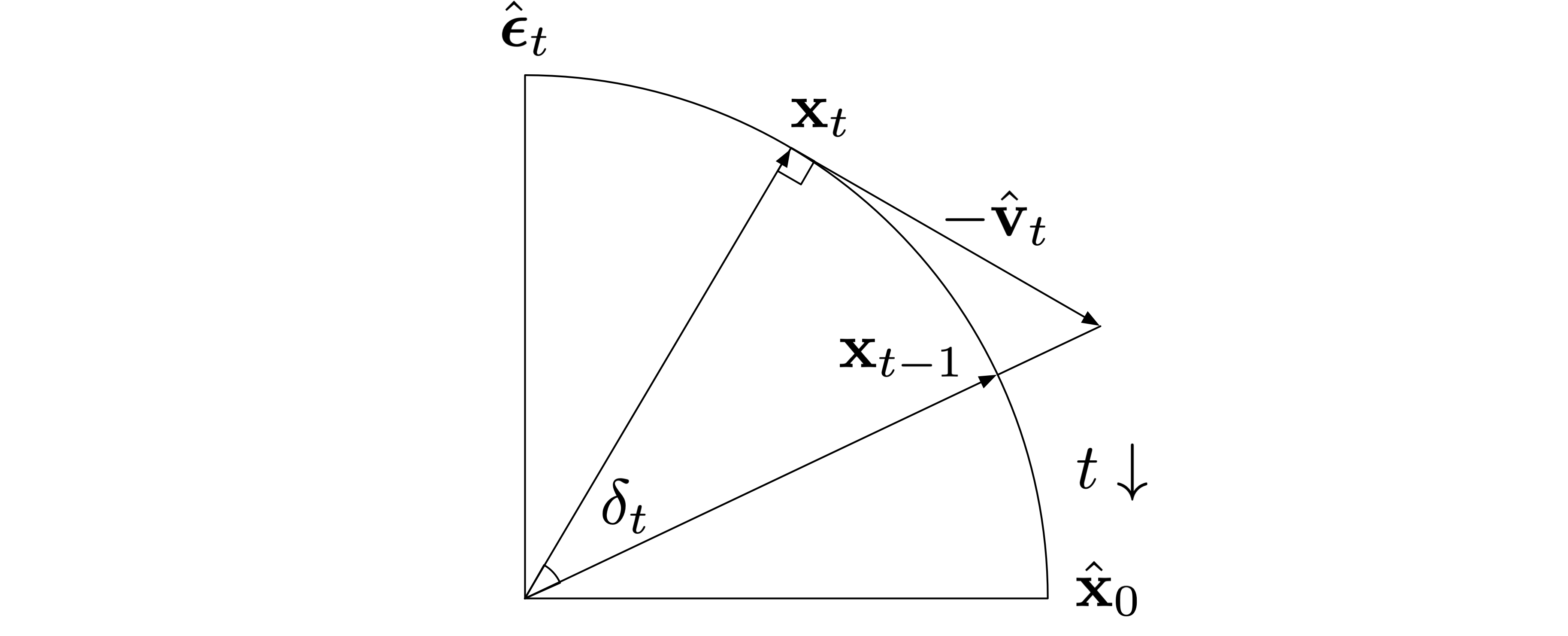
Proof. Recall from the previous section that when \(\gamma_t=0\), given \(\mathbf{x}_t\) we have a deterministic computation for \(\mathbf{x}_{t-1}\) in the forward model. Then we substitute the identities derived previously on the second line below and collect terms on the third line. After converting to angular representations on the fourth line, we apply a few trigonometric identities on the fifth line. \[ \begin{align*} \mathbf{x}_{t-1} & = \alpha_{t-1}\hat{\mathbf{x}}_0(\mathbf{x}_t) + \sigma_{t-1}\hat{\boldsymbol{\epsilon}}_t(\mathbf{x}_t)\\ & = \alpha_{t-1}(\alpha_t\mathbf{x}_t -\sigma_t\hat{\mathbf{v}}_t(\mathbf{x}_t))+\sigma_{t-1}(\sigma_t\mathbf{x}_t+\alpha_t\hat{\mathbf{v}}_t(\mathbf{x}_t))\\ & = (\alpha_{t-1}\alpha_t+\sigma_{t-1}\sigma_t)\mathbf{x}_t + (\alpha_t\sigma_{t-1}-\alpha_{t-1}\sigma_t)\hat{\mathbf{v}}_t(\mathbf{x}_t)\\ & = (\cos\theta_{t-1}\cos\theta_t + \sin\theta_{t-1}\sin\theta_t)\mathbf{x}_t + (\cos\theta_t\sin\theta_{t-1}-\cos\theta_{t-1}\sin\theta_t)\hat{\mathbf{v}}_t(\mathbf{x}_t)\\ & = \cos(\theta_t-\theta_{t-1})\mathbf{x}_t -\sin(\theta_t-\theta_{t-1})\hat{\mathbf{v}}_t(\mathbf{x}_t)\\ & = \cos(\delta_t)\mathbf{x}_t-\sin(\delta_t)\hat{\mathbf{v}}_t(\mathbf{x}_t)\\ \mathbf{x}_{t-1}-\mathbf{x}_t & = (\cos(\delta_t)-1)\mathbf{x}_t-\sin(\delta_t)\hat{\mathbf{v}}_t(\mathbf{x}_t)\\ \end{align*} \]

Taking the limit of both sides after dividing by \(\delta_t\) concludes the proof.

Signal to Noise Ratio

Because \(\boldsymbol\alpha\) and \(\boldsymbol\sigma\) can always be derived from one another, we can also intepret the noise schedule as the specification for a series of monotonic signal-to-noise ratios, defined \[ \begin{align*} \mathrm{SNR}_t & \triangleq \alpha_t^2 / \sigma_t^2\\ \log\mathrm{SNR}_t &= 2(\log\alpha_t - \log\sigma_t) \end{align*} \]

Result. There are a couple helpful identities involving the signal-to-noise ratio. \[ \begin{align*} \alpha_t^2 & = \frac{1}{1 + e^{-\log \mathrm{SNR}_t}} = \mathrm{sigmoid}(\log\mathrm{SNR}_t)\\ \sigma_t^2 & = \frac{1}{1+e^{\log\mathrm{SNR}_t}} = \mathrm{sigmoid}(-\log\mathrm{SNR}_t) \end{align*} \] Proof. This is easy from re-arranging the definition above, using the assumption \(\alpha_t^2+\sigma_t^2 = 1\). \[ \begin{align*} \log \text{SNR}_t & = \log \frac{\alpha_t^2}{1-\alpha_t^2}\\ e^{-\log\text{SNR}_t} & = \frac{1-\alpha_t^2}{\alpha_t^2}\\ \alpha_t^2 & = \frac{1}{1+e^{-\log\mathrm{SNR}_t}} \end{align*} \] The proof for \(\sigma_t^2\) is analogous.

The signal-to-noise ratio arises in a couple of different contexts we'll next discuss.

Min-SNR Weighting

This is an up-weighting strategy very effective in practice (Hang et al. 2023). It's defined as applying a weighting on each term in the ELBO by \[ \begin{align*} \frac{1}{\omega_t}\min(\mathrm{SNR}_t, c),\quad c\triangleq 5. \end{align*} \] In the case of \(\mathbf{x}_0\) parameterization, it's just the familiar squared loss with an additional \(\min(\mathrm{SNR}_t,c)\) weighting. It can be converted to other parameterziations as below. \[ \begin{align*} (\mathbf{x}_0\text{ parameterization})\quad& L'_t(\mathbf{x}_0) = \min(\text{SNR}_t, c)\mathbb{E}_{\tilde{\mathbf{x}}_t\sim q(\mathbf{x}_t|\mathbf{x}_0)}\left\|\mathbf{x}_0 - f_\theta(\tilde{\mathbf{x}}_t)\right\|^2\\ (\boldsymbol\epsilon \text{ parameterization})\quad & L'_t(\mathbf{x}_0) = \min(c/\text{SNR}_t, 1) \mathbb{E}_{\tilde{\mathbf{x}}_t\sim q(\mathbf{x}_t|\mathbf{x}_0)}\left\|\boldsymbol\epsilon - g_\theta(\tilde{\mathbf{x}}_t)\right\|^2\\ (\mathbf{v} \text{ parameterization})\quad & L'_t(\mathbf{x}_0) = \min(\alpha_t^2,c /\sigma_t^2)\mathbb{E}_{\tilde{\mathbf{x}}_t\sim q(\mathbf{x}_t|\mathbf{x}_0)}\left\|\mathbf{v} - h_\theta(\tilde{\mathbf{x}}_t)\right\|^2\\ \end{align*} \] Recall that when using simple losses, \(\boldsymbol\epsilon_t\) prediction is equivalent to \(\mathbf{x}_0\) prediction but weighting by a factor of the SNR. So this can be thought of as an approximation to using the \(\boldsymbol\epsilon_t\) prediction weighting factor, but clamped so that there isn't too much focus in the high SNR regime.

Shifting the Log-SNR for Higher Resolution

Typically the noise schedule is tuned for each dataset, say CIFAR (32 x 32) or ImageNet (64 x 64).

One challenge is how to scale up to larger resolutions, for example ImageNet (512 x 512).

The issue here is that images have highly correlated pixels. Specifically, there's increasingly redundant information from neighboring pixels as the resolution increases. This is evident in the figure below, in which the same amount of noise \(\sigma=0.5\) is applied to an image at various resolutions. Intuitively, more information is destroyed at lower resolutions with the same amount of noise.

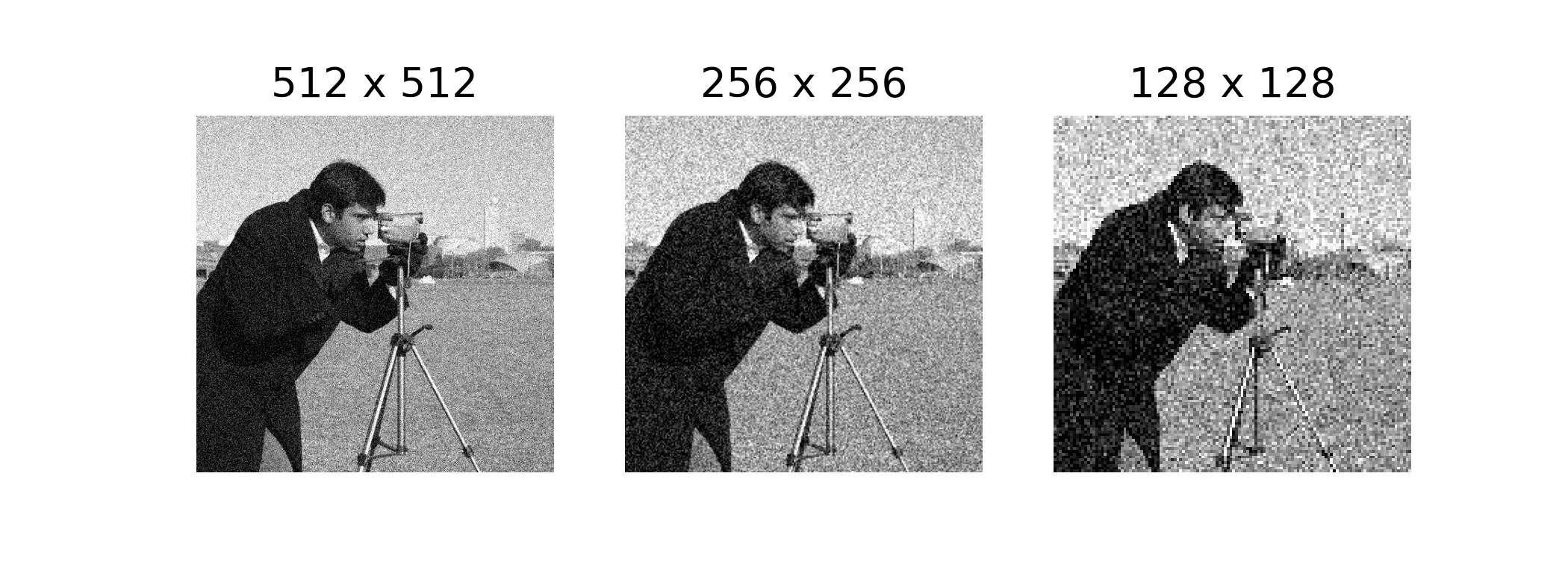
To account for this intuition, Hoogeboom et al. 2023 proposed tuning the noise schedule as a shift in the log-SNR. Specifically, they shift by a factor of \(+2\log\kappa\) where \(\frac{1}{\kappa}\) is the image scale factor (ex. \(\kappa = \frac{1}{2}\) to go from 64 x 64 to 128 x 128).

Conversion back into \(\alpha_t,\sigma_t\) can be made by using the identities we saw earlier. \[ \begin{align*} \alpha_t^2 & = \text{sigmoid}(\log\mathrm{SNR}_t +2\log\kappa)\\ \sigma_t^2 & = \text{sigmoid}(-\log\mathrm{SNR}_t -2\log\kappa)\\ \end{align*} \] An equivalent (yet more intuitive method) proposed by Chen 2023 is to pre-process the inputs such that they're scaled by \(\kappa\) (for example, \(\kappa=\frac{1}{2}\)). This makes sense because by lowering the amount of signal in each pixel, it's harder to reconstruct the original image given the same level of noise.

Result. Pre-processing the input by a scale \(\kappa\) is equivalent to a shift in the log-SNR by \(+2 \log\kappa\).

Proof. The variance of a Monte Carlo sample used at training time is, \[ \begin{align*} \mathrm{Var}[\tilde{\mathbf{x}}_t] & = \mathrm{Var}[\alpha_t\kappa\mathbf{x}_0 + \sigma_t\boldsymbol\epsilon_t]\\ & = \alpha_t^2\kappa^2\mathrm{Var}[\mathbf{x}_0]+ \sigma_t^2\mathbf{I}\\ & = (\alpha_t^2\kappa^2+\sigma_t^2)\mathbf{I} \end{align*} \] where on the last line we made the assumption that \(\mathrm{Var}[\mathbf{x}_0]= \mathbf{I}\). The log-SNR is then \[ \begin{equation*} \log \frac{\alpha_t^2\kappa^2}{\sigma_t^2} = 2(\log \alpha_t -\log \sigma_t+ \log \kappa). \end{equation*} \]

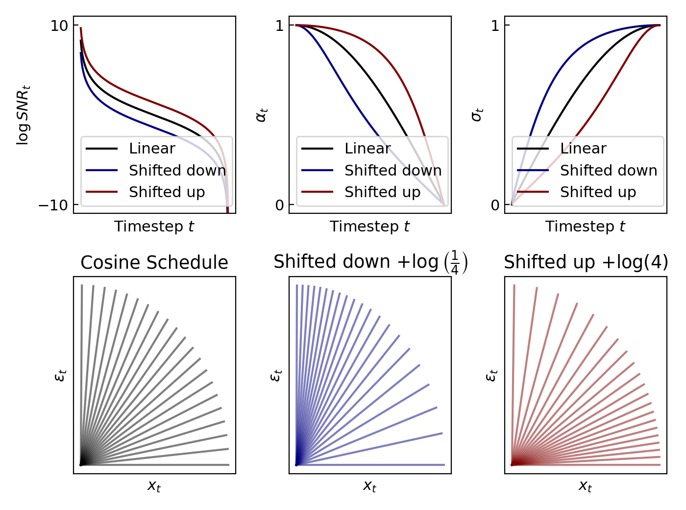
In the figure below, we compare the effect of shifting down/up the default cosine schedule. In the first row we show how the coefficients \(\alpha_t,\sigma_t\) are affected. In the second row we show the angular interpretation of each of the corresponding noise schedules.

[Footnote 1]. The cosine schedule is typically approximated with the following equations for numerical reasons, where \(s=0.008\). \[ \begin{align*} \alpha_t^2 = \frac{f_t}{f_0},\quad\quad f_t = \cos\left(\frac{t/T+s}{1+s}\frac{\pi}{2}\right)^2 \end{align*} \]