IV. Sampling
In this section we'll discuss various considerations at sampling time. After reading this page (particularly the "Accelerated Sampling" section) you should be able to understand everything in the "simple" implementation in the codebase [here].
Accelerated Sampling
It's straightforward to sample the forward process by sampling from \(p(\mathbf{x}_T)\), then \(p_\theta(\mathbf{x}_{t-1}|\mathbf{x}_t)\), so on and so forth until we draw a sample \(p(\mathbf{x}_0)\).
But this is extremely slow when \(T\) is large. How can we speed it up?
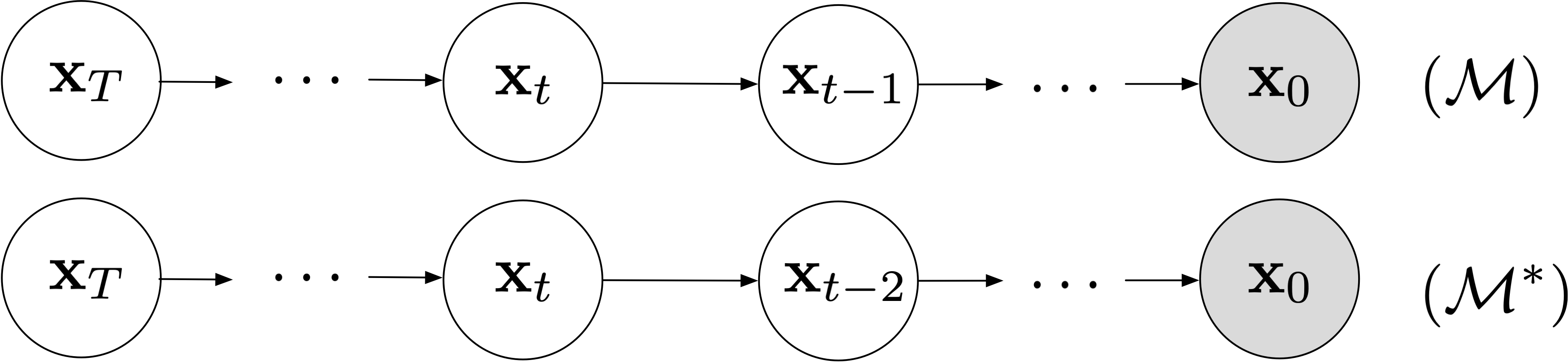
Setup. The approach we'll take is sampling with striding. For the sake of concreteness, in the rest of this section we'll assume we want to sample every other latent variable (assume \(T\) is even). That is, we want to start from \(\mathbf{x}_T\), then sample \(\mathbf{x}_{T-2}\), then \(\mathbf{x}_{T-4}\), and so on until \(\mathbf{x}_2\) and \(\mathbf{x}_0\).
(Generalization to other, potentially non-uniform striding choices is straightforward.)
One attempt would be to compute \(q(\mathbf{x}_{t-2}|\mathbf{x}_t,\mathbf{x}_0)\) on \(\mathcal{M}\). But the integral here is intractable to compute, especially for arbitrary striding.
\[ \begin{align*} q(\mathbf{x}_{t-2}|\mathbf{x}_t,\mathbf{x}_0) & = \int_{\mathbf{x}_{t-1}}q(\mathbf{x}_{t-2},\mathbf{x}_{t-1}|\mathbf{x}_{t},\mathbf{x}_{0})d\mathbf{x}_{t-1}\\ & = \int_{\mathbf{x}_{t-1}}q(\mathbf{x}_{t-2}|\mathbf{x}_{t-1},\mathbf{x}_0)q(\mathbf{x}_{t-1}|\mathbf{x}_{t},\mathbf{x}_{0})d\mathbf{x}_{t-1} \end{align*} \]
Instead, we can hypothesize an alternative graphical model to the one we've been using.
Define. We define the graphical model \(\mathcal{M}^\ast\) in which only even-indexed variables for a Markov chain and the odd-indexed variables are no longer involved.
The key here is that we'll make distributional assumptions so that \(\mathcal{M}^\ast\) has the same marginal distributions (conditioned on \(\mathbf{x}_0\)) as \(\mathcal{M}\). Specifically, we'll assume the following forward and backward models, where once again we use Bayes' Rule to express the backward model more conveniently. \[ \begin{align*} p(\mathbf{x}_{0:T}) & = p(\mathbf{x}_T)\prod_{t\text{ even}} p_\theta(\mathbf{x}_{t-2}|\mathbf{x}_t)\\ q(\mathbf{x}_{1:T}|\mathbf{x}_0) & = \prod_{t \text{ even}}q(\mathbf{x}_{t}|\mathbf{x}_{t-2},\mathbf{x}_0)\\ & = \prod_{t \text{ even}}\frac{q(\mathbf{x}_{t-2}|\mathbf{x}_{t},\mathbf{x}_0)q(\mathbf{x}_t|\mathbf{x}_0)}{q(\mathbf{x}_{t-2}|\mathbf{x}_0)}\\ & = q(\mathbf{x}_T|\mathbf{x}_0)\prod_{t\text{ even}}q(\mathbf{x}_{t-2}|\mathbf{x}_t,\mathbf{x}_0) \end{align*} \]
Then we can define, similar to the standard setup, backward and forward models respectively as \[ \begin{align*} q(\mathbf{x}_{t-2}|\mathbf{x}_t,\mathbf{x}_0) & = N\left(\alpha_{t-2}\mathbf{x}_0 + \sqrt{\sigma_{t-2}^2 - \gamma_t^2}\frac{\mathbf{x}_t-\alpha_t\mathbf{x}_0}{{\sigma_t}}, \gamma_t^2 \mathbf{I}\right)\\ p_\theta(\mathbf{x}_{t-2}|\mathbf{x}_t) & = q(\mathbf{x}_{t-2}|\mathbf{x}_t,f_\theta(\mathbf{x}_t)). \end{align*} \] Result. If we repeat the math previously derived but for \(\mathcal{M}^\ast\), we can verify that the marginal distributions of variables (conditioned on \(\mathbf{x}_0\)) match the original model \(\mathcal{M}\). That is, for all \(t\) the key result holds, \[ \begin{align*} q(\mathbf{x}_t|\mathbf{x}_0) = N(\alpha_t \mathbf{x}_0, \sigma_t ^2\mathbf{I}). \end{align*} \] Moreover, the Evidence Lower Bound will be very similar to the previous setup, \[ \begin{align*} L(\mathbf{x}_0) & = \underbrace{\mathbb{E}_{q(\mathbf{x}_2|\mathbf{x}_0)}\left[\log p_\theta(\mathbf{x}_0|\mathbf{x}_2)\right]}_{\text{ignored}} - \sum_{t>2 \text{ even}} \underbrace{\mathbb{E}_{q(\mathbf{x}_t|\mathbf{x}_0)}\left[D_\mathrm{KL}(\ q(\mathbf{x}_{t-2}|\mathbf{x}_t, \mathbf{x}_0)\ \|\ p_\theta(\mathbf{x}_{t-2}|\mathbf{x}_t)\ )\right]}_{L_t(\mathbf{x}_0)}\\ L_t(\mathbf{x}_0) & = \mathbb{E}_{\tilde{\mathbf{x}}_t\sim q(\mathbf{x}_t|\mathbf{x}_0)}\left[D_\mathrm{KL}(\ \underbrace{q(\mathbf{x}_{t-2}|\tilde{\mathbf{x}}_t, \mathbf{x}_0)}_{\text{groundtruth}}\ \|\ \underbrace{p_\theta(\mathbf{x}_{t-2}|\tilde{\mathbf{x}}_t)}_\text{prediction}\ )\right]\\ & = \underbrace{\frac{1}{2\gamma_t^2}\left(\alpha_{t-1}-\frac{\alpha_t}{\sigma_t}\sqrt{\sigma_{t-1}^2-\gamma_t^2}\right)^2}_{\omega_t}\mathbb{E}_{\tilde{\mathbf{x}}_t\sim q(\mathbf{x}_t|\mathbf{x}_0)}\left\|\mathbf{x}_0 - f_\theta(\tilde{\mathbf{x}}_t)\right\|^2\\ & = \omega_t\mathbb{E}_{\tilde{\mathbf{x}}_t\sim q(\mathbf{x}_t|\mathbf{x}_0)}\left\|\mathbf{x}_0 - f_\theta(\tilde{\mathbf{x}}_t)\right\|^2 \end{align*} \] There are two differences between the losses resulting from \(\mathcal{M}^\ast\) compared to \(\mathcal{M}\).
- There are only \(L_t\) terms corresponding to even values of \(t\) and not odd values of \(t\). This means that at training time we are supervising with extra Monte Carlo samples \(\tilde{\mathbf{x}}_t\) and losses corresponding to odd \(t\). We can justify this as a kind of regularization with data augmentation.
- The weighting factor out front i.e. \(\omega_t\) is slightly different. However, this is justified by the fact that we're typically training with the simplified objectives anyway which ignore these weighting coefficients. This can be interpreted as optimization of a re-weighted Evidence Lower Bound.
Choice of Backward Variance
So far we have ignored the role of hyper-parameter \(\boldsymbol\gamma\). How does it play a role?
Training Time
\(\gamma_t\) is typically ignored. This is because the simple losses we defined previously have no dependence on it.
Where \(\gamma_t\) does play a role is in the case where we want to optimize the actual ELBO instead of a simple loss. Recall that the ELBO is a weighted version of the simple loss which involves the weighting coefficient that depends on \(\gamma_t\) via
\[ \begin{align*} \omega_t = \frac{1}{2\gamma_t^2}\left(\alpha_{t-1}-\frac{\alpha_t}{\sigma_t}\sqrt{\sigma_{t-1}^2-\gamma_t^2}\right)^2. \end{align*} \] However, this is rarely done in the literature; nearly everybody ignores the role of \(\gamma_t\) at training time. This gives us flexibility to choose \(\gamma_t\) at evaluation time post-hoc, after already having a trained model.
Evaluation Time
Typically \(\gamma_t = 0\) for all values of \(t\). Recall the definition of the forward model, \[ \begin{align*} p_\theta(\mathbf{x}_{t-1}|\mathbf{x}_t) & = q(\mathbf{x}_{t-1}|\mathbf{x}_t,f_\theta(\mathbf{x}_t))\\ & = N\left(\alpha_{t-1}f_\theta(\mathbf{x}_t) + \sqrt{\sigma_{t-1}^2 - \gamma_t^2}\frac{\mathbf{x}_t-\alpha_tf_\theta(\mathbf{x}_t)}{{\sigma_t}}, \gamma_t^2 \mathbf{I}\right). \end{align*} \] So by decreasing \(\gamma_t\) to a value as low as possible we are actually making the model deterministic conditioned on \(\mathbf{x}_T\) (i.e. an implicit generative model arises). There is no longer any stochasticity between latent variables and there is a fixed mapping between \(\mathbf{x}_0 \leftrightarrow \mathbf{x}_T\).
We can then write the forward sampling process in this setup as \[ \begin{align*} \mathbf{x}_{T} & \sim N(\mathbf{0},\mathbf{I})\\ \text{iterate }\mathbf{x}_{t-1} &= \alpha_{t-1}f_\theta(\mathbf{x}_{t}) + \sigma_{t-1}\frac{\mathbf{x}_{t}-\alpha_t f_\theta(\mathbf{x}_t)}{\sigma_t}\\ & = \alpha_{t-1}\hat{\mathbf{x}}_0(\mathbf{x}_t) + \sigma_{t-1}\hat{\boldsymbol{\epsilon}}_t(\mathbf{x}_t), \end{align*} \]
where \(\hat{\mathbf{x}}_0\) and \(\hat{\boldsymbol{\epsilon}}_t\) can be derived from any choice of neural network parameterization (see previous section) and these are computed as a function of \(\mathbf{x}_t\) on each sampling iteration.
Guidance
The most common way to improve generation quality is via classifier-free guidance.
In this setup, we are given labeled categorical data \(\{\mathbf{x}^{(i)}, y^{(i)}\}\) with \(K\) classes.
Classifier Guidance
Suppose we can train an auxiliary classifier \(p_\phi(y|\mathbf{x})\) to predict the class of an input \(\mathbf{x}\).
For this setup, recall the score matching perspective of the \(\boldsymbol\epsilon\) parameterization. We know that \[ \begin{align*} \hat{\boldsymbol\epsilon}(\mathbf{x}_t) \approx -\sigma_t\nabla_{\mathbf{x}_t}\log q(\mathbf{x}_t|\mathbf{x}_0) \end{align*} \] In the sampling process, we're going to alter the score by guiding it, taking the gradient of the auxiliary classifier into account (Dhariwal and Nichol 2021). Specifically, we can define an altered distribution \[ \begin{align*} q'(\mathbf{x}_t|\mathbf{x}_0) & \propto q(\mathbf{x}_t|\mathbf{x}_0)p_\phi(y|\mathbf{x}_t)^w \end{align*} \] for some arbitrary constant \(w > 0\) (roughly on the order of \(w\approx 5\) usually works okay).
Then the score of this altered distribution is \[ \begin{align*} \nabla_{\mathbf{x}_t}\log q'(\mathbf{x}_t|\mathbf{x}_0) & = \nabla_{\mathbf{x}_t}\log q(\mathbf{x}_t|\mathbf{x}_0) + w\nabla_{\mathbf{x}_t}\log p_\phi(y|\mathbf{x}_t)\\ &\approx -\frac{1}{\sigma_t} \hat{\boldsymbol\epsilon}(\mathbf{x}_t) + w \nabla_{\mathbf{x}_t}\log p_\phi(y|\mathbf{x}_t)\\ & = -\frac{1}{\sigma_t}\underbrace{\left(\hat{\boldsymbol\epsilon}(\mathbf{x}_t)- w\sigma_t\nabla_{\mathbf{x}_t}\log p_\phi(y|\mathbf{x}_t)\right)}_{\hat{\boldsymbol\epsilon}'(\mathbf{x}_t)}. \end{align*} \]
We can plug in the altered \(\hat{\boldsymbol\epsilon}'(\mathbf{x}_t)\) in the forward process to draw samples from the guided distribution.
Intuitively, this will be guiding the gradients of the distribution toward the class-specific mode.
Classifier-Free Guidance
The idea here is to hypothesize conditioning the auxiliary classifier on \(\mathbf{x}_0\), then use Bayes' Rule to invert the classifier into a generative model (Ho and Salimans 2022). First, we note that in this setup we model the class-conditional distribution \(p_\mathrm{data}(\mathbf{x}_0|y)\) by conditioning the neural network approximation on labels, \[ \begin{align*} \hat{\boldsymbol\epsilon}(\mathbf{x}_t,y) \approx -\sigma_t \nabla_{\mathbf{x}_t}\log q(\mathbf{x}_t|\mathbf{x}_0,y) \end{align*} \] Then suppose our auxiliary classifier is instead formulated as follows. \[ \begin{align*} p_\phi(y|\mathbf{x}_t,\mathbf{x}_0) & = \frac{p_\phi(\mathbf{x}_t|\mathbf{x}_0,y)p(y|\mathbf{x}_0)}{p_\phi(\mathbf{x}_t|\mathbf{x}_0)} \tag{Bayes' Rule}\\ \nabla_{\mathbf{x}_t}\log p_\phi(y|\mathbf{x}_t,\mathbf{x}_0) & = \underbrace{\nabla_{\mathbf{x}_t}\log p_\phi(\mathbf{x}_t|\mathbf{x}_0,y)}_{-\hat{\boldsymbol\epsilon}_t(\mathbf{x}_t,y)/\sigma_t} - \underbrace{\nabla_{\mathbf{x}_t}\log p_\phi(\mathbf{x}_t|\mathbf{x}_0)}_{-\hat{\boldsymbol\epsilon}_t(\mathbf{x}_t,\varnothing)/\sigma_t} \end{align*} \] We're going to choose to
- Model \(\nabla_{\mathbf{x}_t}\log p_\phi(\mathbf{x}_t|\mathbf{x}_0,y)\) with the same score network estimate \(\hat{\boldsymbol{\epsilon}}_t\) for \(\nabla_{\mathbf{x}_t}\log q(\mathbf{x}_t|\mathbf{x}_0,y)\)
- Model \(\nabla_{\mathbf{x}_t}\log p_\phi(\mathbf{x}_t|\mathbf{x}_0)\) with the same score network, but where we drop out the label and feed in a null token \(\varnothing\). At training time, this corresponds to dropping out the label a fraction of the time.
Putting it together, the score of the altered distribution will be \[ \begin{align*} \nabla_{\mathbf{x}_t}\log q'(\mathbf{x}_t|\mathbf{x}_0,y) & = \nabla_{\mathbf{x}_t}\log q(\mathbf{x}_t|\mathbf{x}_0,y) + w\nabla_{\mathbf{x}_t}\log p_\phi(y|\mathbf{x}_t,\mathbf{x}_0)\\ &\approx -\frac{1}{\sigma_t} \hat{\boldsymbol\epsilon}(\mathbf{x}_t,y) + w \left(-\frac{1}{\sigma_t}\hat{\boldsymbol\epsilon}(\mathbf{x}_t,y) + \frac{1}{\sigma_t}\hat{\boldsymbol\epsilon}(\mathbf{x}_t,\varnothing)\right)\\ &= -\frac{1}{\sigma_t}\underbrace{\left((1+w)\hat{\boldsymbol\epsilon}(\mathbf{x}_t,y)- w\hat{\boldsymbol\epsilon}(\mathbf{x}_t,\varnothing)\right)}_{\hat{\boldsymbol\epsilon}''(\mathbf{x}_t,y)\\} \end{align*} \] We can plug in the altered \(\hat{\boldsymbol\epsilon}''(\mathbf{x}_t)\) in the forward process to draw samples from the guided distribution.