Home

[Return to Index]

I. Structure

A diffusion model hypothesizes an observed variable \(\mathbf{x}_0\) and latent variables \(\mathbf{x}_1,\dots,\mathbf{x}_T\) arranged in the following graphical model.

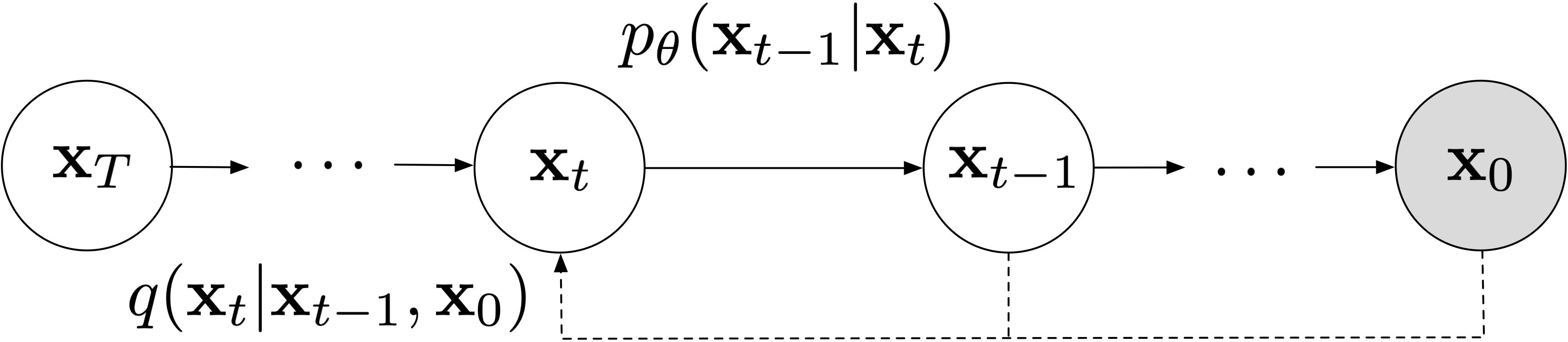
We assume the following forward and backward models respectively. \[ \begin{align*} p_\theta(\mathbf{x}_{0:T}) & = p(\mathbf{x}_T)\prod_{t>0} p_\theta(\mathbf{x}_{t-1}|\mathbf{x}_t)\\ q(\mathbf{x}_{1:T}|\mathbf{x}_0) & = \prod_{t>0} q(\mathbf{x}_t|\mathbf{x}_{t-1},\mathbf{x}_0)\\ & = \prod_{t>0} \frac{q(\mathbf{x}_{t-1}|\mathbf{x}_t,\mathbf{x}_0)q(\mathbf{x}_t|\mathbf{x}_0)}{q(\mathbf{x}_{t-1}|\mathbf{x}_0)}\\ & = q(\mathbf{x}_T|\mathbf{x}_0) \prod_{t>1} q(\mathbf{x}_{t-1}|\mathbf{x}_t,\mathbf{x}_0). \end{align*} \]

The re-arranging to arrive at the last line above follows from Bayes' Rule. For our purposes, it will usually be more convenient to describe the backward process via the latter representation rather than the former.

In later sections we'll define specific distributional assumptions. But for now it suffices to note the following.

Remark. The backward model \(q(\mathbf{x}_{1:T}|\mathbf{x}_0)\) is fixed. All learnable parameters lie in the forward model \(p_\theta(\mathbf{x}_{t-1}|\mathbf{x}_t)\).

Remark. The forward model is Markovian. The backward model is Markovian when conditioned on \(\mathbf{x}_0\).

Remark. It's straightforward to draw a sample \(\mathbf{x}_0\) from the forward model. We first sample \(\mathbf{x}_T\) from the unconditional prior, then \(\mathbf{x}_{t-1}\) conditioned on \(\mathbf{x}_t\), and so on until we sample \(\mathbf{x}_0\) conditioned on \(\mathbf{x}_1\) ("ancestral sampling"). So inference time is uncomplicated. Our focus in the next few sections will be on what happens at training time.

Remark. Our presentation here follows the DDIM paper (Song et al. 2021) which generalizes earlier work in the DDPM paper (Ho et al. 2020). That is, DDPM is a specific instantiation of DDIM with stronger assumptions. We'll devote a page to discussing this later on.

The Evidence Lower Bound

As with any latent-variable model, the training objective is to maximize marginal log-likelihood.

\[ \begin{align*} \log p_\theta(\mathbf{x}_0) & = \log \int_{\mathbf{x}_{1:T}} p_\theta(\mathbf{x}_0,\mathbf{x}_{1:T})d\mathbf{x}_{1:T} \end{align*} \]

But this is intractable to compute due to the integral over unobserved variables. Instead we'll maximize the Evidence Lower Bound (ELBO) which arises from Jensen's inequality.

\[ \begin{align*} \log p_\theta(\mathbf{x}_0) & = \log \int_{\mathbf{x}_{1:T}} p_\theta(\mathbf{x}_0,\mathbf{x}_{1:T})d\mathbf{x}_{1:T}\\ & = \log \int_{\mathbf{x}_{1:T}}q(\mathbf{x}_{1:T}|\mathbf{x}_0)\frac{p_\theta(\mathbf{x}_0,\mathbf{x}_{1:T})}{q(\mathbf{x}_{1:T}|\mathbf{x}_0)}d\mathbf{x}_{1:T}\\ & \geq \int_{\mathbf{x}_{1:T}}q(\mathbf{x}_{1:T}|\mathbf{x}_0)\log \frac{p_\theta(\mathbf{x}_0,\mathbf{x}_{1:T})}{q(\mathbf{x}_{1:T}|\mathbf{x}_0)}d\mathbf{x}_{1:T} \triangleq L_\theta(\mathbf{x}_0) \end{align*} \]

Why is this a reasonable quantity to optimize?

Result. The gap between the marginal log-likelihood and the ELBO is exactly the KL divergence between the true forward model \(p_\theta(\mathbf{x}_{1:T}|\mathbf{x}_0)\) (which is intractable) and the hypothesized backward model \(q(\mathbf{x}_{1:T}|\mathbf{x}_0)\). So by maximizing the ELBO we're optimizing how well we approximate the hypothesized backward model.

Proof. Let's compute the gap between the marginal likelihood and the ELBO. \[ \begin{align*} \log p_\theta(\mathbf{x_0}) - L_{\theta}(\mathbf{x_0}) & = \log \int_{\mathbf{x}_{1:T}} p_\theta(\mathbf{x}_0,\mathbf{x}_{1:T}) d\mathbf{x}_{1:T} - \int_{\mathbf{x}_{1:T}} q(\mathbf{x}_{1:T}|\mathbf{x}_0) \log \frac{p_\theta(\mathbf{x}_0)p_\theta(\mathbf{x}_{1:T}|\mathbf{x}_0)}{q(\mathbf{x}_{1:T}|\mathbf{x}_0)}d\mathbf{x}_{1:T}\\ & = \log \int_{\mathbf{x}_{1:T}} p_\theta(\mathbf{x}_{1:T}|\mathbf{x}_0) d\mathbf{x}_{1:T} + \log p_\theta(\mathbf{x}_0) - \int_{\mathbf{x}_{1:T}} q_\phi(\mathbf{x}_{1:T}|\mathbf{x}_0) \log \frac{p_\theta(\mathbf{x}_{1:T}|\mathbf{x}_0)}{q_\phi(\mathbf{x}_{1:T}|\mathbf{x}_0)}d\mathbf{x}_{1:T} - \log p_\theta(\mathbf{x}_0)\\ & = \underbrace{\log \int_{\mathbf{x}_{1:T}} p_\theta(\mathbf{x}_{1:T}|\mathbf{x}_0) d\mathbf{x}_{1:T}}_{\varnothing} - \int_{\mathbf{x}_{1:T}} q_\phi(\mathbf{x}_{1:T}|\mathbf{x}_0) \log \frac{p_\theta(\mathbf{x}_{1:T}|\mathbf{x}_0)}{q_\phi(\mathbf{x}_{1:T}|\mathbf{x}_0)}d\mathbf{x}_{1:T} \\ & = D_\mathrm{KL}(\ q_\phi(\mathbf{x}_{1:T}|\mathbf{x}_0)\ \|\ p_\theta(\mathbf{x}_{1:T}|\mathbf{x}_0)\ ) \geq 0 \end{align*} \]

On the last line above we invoked the non-negativity of KL divergence.

Result. From the structure of the graphical model assumed, we will be able to simplify the ELBO into a convenient form. \[ \begin{align*} L_\theta(\mathbf{x}_0) & = \int_{q(\mathbf{x}_{1:T}|\mathbf{x}_0)} \prod_{t=1}^Tq(\mathbf{x}_t|\mathbf{x}_{t-1}) \log \frac{p(\mathbf{x}_T)\prod_{t>0} p_\theta(\mathbf{x}_{t-1}|\mathbf{x}_t)}{q(\mathbf{x}_T|\mathbf{x}_0)\prod_{t>1} q(\mathbf{x}_{t-1}|\mathbf{x}_{t},\mathbf{x}_0)}d\mathbf{x}_{1:T}\\ & = \mathbb{E}_{q(\mathbf{x}_{1:T}|\mathbf{x}_0)}\left[\log \frac{p(\mathbf{x}_T)}{q(\mathbf{x}_T|\mathbf{x}_0)} + \log p_\theta(\mathbf{x}_0|\mathbf{x}_1)+ \sum_{t>1} \log p_\theta(\mathbf{x}_{t-1}|\mathbf{x}_t) -\sum_{t>1}\log q(\mathbf{x}_{t-1}|\mathbf{x}_{t},\mathbf{x}_0) \right]\\ & = \mathbb{E}_{q(\mathbf{x}_{1:T}|\mathbf{x}_0)}\left[\log \frac{p(\mathbf{x}_T)}{q(\mathbf{x}_T|\mathbf{x}_0)} + \sum_{t>1} \log \frac{p_\theta(\mathbf{x}_{t-1}|\mathbf{x}_t)}{q(\mathbf{x}_{t-1}|\mathbf{x}_t,\mathbf{x}_0)} + \log p_\theta(\mathbf{x}_0|\mathbf{x}_1)\right]\\ & = \mathbb{E}_{q(\mathbf{x}_T|\mathbf{x}_0)}\left[\log \frac{p(\mathbf{x}_T)}{q(\mathbf{x}_T|\mathbf{x}_0)}\right] + \sum_{t>1}\mathbb{E}_{q(\mathbf{x}_{t-1},\mathbf{x}_t|\mathbf{x}_0)}\left[\log\frac{p_\theta(\mathbf{x}_{t-1}|\mathbf{x}_t)}{q(\mathbf{x}_{t-1}|\mathbf{x}_t,\mathbf{x}_0)}\right] + \mathbb{E}_{q(\mathbf{x}_1|\mathbf{x}_0)}\left[\log p_\theta(\mathbf{x}_0|\mathbf{x}_1)\right]\\ & = \mathbb{E}_{q(\mathbf{x}_1|\mathbf{x}_0)}\left[\log p_\theta(\mathbf{x}_0|\mathbf{x}_1)\right] - \sum_{t>1}\mathbb{E}_{q(\mathbf{x}_t|\mathbf{x}_0)}\left[D_\mathrm{KL}(\ q(\mathbf{x}_{t-1}|\mathbf{x}_t, \mathbf{x}_0)\ \|\ p_\theta(\mathbf{x}_{t-1}|\mathbf{x}_t)\ )\right] -D_\mathrm{KL}(\ q(\mathbf{x}_T|\mathbf{x}_0)\ \|\ p(\mathbf{x}_T)\ )\\ & \propto \underbrace{\mathbb{E}_{q(\mathbf{x}_1|\mathbf{x}_0)}\left[\log p_\theta(\mathbf{x}_0|\mathbf{x}_1)\right]}_{L_1(\mathbf{x}_0)} - \sum_{t>1} \underbrace{\mathbb{E}_{q(\mathbf{x}_t|\mathbf{x}_0)}\left[D_\mathrm{KL}(\ q(\mathbf{x}_{t-1}|\mathbf{x}_t, \mathbf{x}_0)\ \|\ p_\theta(\mathbf{x}_{t-1}|\mathbf{x}_t)\ )\right]}_{L_t(\mathbf{x}_0)} \end{align*} \]

Above we used the fact that there are no learnable parameters in \(D_\mathrm{KL}(\ q(\mathbf{x}_T|\mathbf{x}_0)\ \|\ p(\mathbf{x}_T)\ )\).

Remark. The \(L_1(\mathbf{x}_0)\) term is typically considered unimportant and the focus will be on optimizing \(L_t(\mathbf{x}_0)\).

The last line is important because it makes the expectations explicit (for whatever reason most references I find online omit this detail, which I find crucial for understanding).

Remark. Each individual term in the ELBO relies only on expectations over factorized conditional distributions \(q(\mathbf{x}_t|\mathbf{x}_0)\) instead of the joint \(q(\mathbf{x}_{1:T}|\mathbf{x}_0)\).

This is important because we'll later optimize the ELBO via Monte Carlo estimates of these expectations, and factorizing in this way makes it tractable. Let us rewrite \(L_t(\mathbf{x}_0)\) and expand it slightly for sake of clarity. \[ \begin{align*} L_t(\mathbf{x}_0) & = \mathbb{E}_{\tilde{\mathbf{x}}_t\sim q(\mathbf{x}_t|\mathbf{x}_0)}\left[D_\mathrm{KL}(\ \underbrace{q(\mathbf{x}_{t-1}|\tilde{\mathbf{x}}_t, \mathbf{x}_0)}_{\text{groundtruth}}\ \|\ \underbrace{p_\theta(\mathbf{x}_{t-1}|\tilde{\mathbf{x}}_t)}_\text{prediction}\ )\right] \end{align*} \] In the next section we'll pick a convenient definition of the backward process \(q(\mathbf{x}_t|\mathbf{x}_0)\) so that \(\tilde{\mathbf{x}}_t\) is easy to sample.

(Quick discussion on notation. Here and throughout the rest of this post, we'll use notation \(\tilde{\mathbf{x}}_t\) to denote a random variable drawn from \(q(\mathbf{x}_t|\mathbf{x}_0)\). This is because the notation \(\mathbf{x}_t\) alone is rather ambiguous, as it can denote a random variable drawn from either the unconditional distribution \(q(\mathbf{x}_t)\) or the conditional distribution \(q(\mathbf{x}_t|\mathbf{x}_0)\). Hopefully this reduces confusion I've seen arise in other references.)

Given a Monte Carlo sample \(\tilde{\mathbf{x}}_t \sim q(\mathbf{x}_t|\mathbf{x}_0)\), the loss will simply be the KL divergence between a fixed groundtruth distribution (as a function of \(\tilde{\mathbf{x}}_t,\mathbf{x}_0\)) and a modeled predictive distribution (as a function of \(\tilde{\mathbf{x}}_t\)).

Pseudocode. By drawing Monte Carlo samples \(\tilde{\mathbf{x}}_t \sim q(\mathbf{x}_t|\mathbf{x}_0)\), we can use the following estimator for \(L_t(\mathbf{x}_0)\), \[ \begin{align*} \tilde{L}_t(\mathbf{x}_0) & = \frac{1}{M} \sum_{m=1}^M D_\mathrm{KL}(\ \underbrace{q(\mathbf{x}_{t-1}|\tilde{\mathbf{x}}_t^{(m)}, \mathbf{x}_0)}_{\text{groundtruth}}\ \|\ \underbrace{p_\theta(\mathbf{x}_{t-1}|\tilde{\mathbf{x}}_t^{(m)})}_\text{prediction}), \quad {\tilde{\mathbf{x}}_t^{(m)} \sim q(\mathbf{x}_t|\mathbf{x}_0)} \end{align*} \] In practice typically \(M=1\). In pseudocode, the algorithm will look something like the following.

def compute_L_t(x_0):
    t = sample_t(lower=1, upper=T)  # amortize the sum over t via samples
    monte_carlo_x_t = sample q(x_t | x_0)  # draw a sample for each example in the batch
    true_distn = get_gt_q_x_t_minus_1(monte_carlo_x_t, x_0, t)
    pred_distn = get_pred_p_x_t_minus_1(monte_carlo_x_t, t)  # gradient flows into model
    loss = compute_kl_div(true_distn, pred_distn)
    return loss

This is reminiscent of the training procedure for a variational auto-encoder (Kingma and Welling 2014). But because there are no learnable parameters in the distribution we're sampling from, i.e. \(q(\mathbf{x}_t|\mathbf{x}_0)\), the re-parameterization trick (or a similar technique such as log-derivative trick) is not even necessary. A simple Monte Carlo sample suffices.

Remark. The formulation here does not readily admit tractable log-likelihood evaluation. This is due to the inability to marginalize over latent variables \(\mathbf{x}_{1:T}\) in the expression for marginal log-likelihood.

For comparison to likelihood-based generative models (such as autoregressive models and normalizing flows), Ho et al. (2020) and Kingma et al. (2021) report likelihood metrics in terms of the ELBO. We'll later see that it is possible to recover exact likelihood calculation via a slightly different ordinary differential equations formulation (Song et al. 2021).